On the cover: A weather forecasting stone meme
Imagine you live, work and vacation in three different cities.
In City A (home), it is sunny every single day. No clouds. No rain. Ever. You wake up, glance outside, and already know the answer. Boring? Yes. Informative? Not at all.
Now consider City B (work). Every morning, the weather could be sunny, rainy, or cloudy, each with equal probability. You actually check the forecast now, because there’s uncertainty involved.
Finally, welcome to City C (vacation). Here, the weather might be sunny, rainy, cloudy, snowing, hailing, stormy, or something you’ve never seen before. Every day feels like a plot twist or surprise.
Guess what changed as we moved from City A to B to C?
The number of possible outcomes increased. But more importantly, the uncertainty about tomorrow increased. Intuitively, the “less certain” or “more surprised” you are about what will happen, the more information the outcome carries.
A forecast that says “it will definitely be sunny” carries almost no information. A forecast that says “it could be anything” carries a lot.
So how do we measure this uncertainty? We need to borrow from Information Theory. What has this got to do with Cross Entropy loss? We’ll get there, please bear with me.
Shannon’s Questions and Axioms
Claude Shannon, often called the father of information theory, asked a deceptively simple question:
“How do we measure information in a way that makes sense?”
He wanted a mathematical quantity that:
- increases when the forecast becomes more unpredictable
- decreases when outcomes become certain
- behaves nicely when we combine independent events
Instead of guessing a formula, Shannon laid down axioms - rules any reasonable measure of uncertainty must follow.
Let’s call our uncertainty measure entropy, denoted by $H(p)$, where $p$ is the probability distribution over weather outcomes.
1. Continuity
If tomorrow’s rain probability changes from 30% to 33%, the uncertainty shouldn’t jump wildly. So, small changes in forecast should reflect small changes in entropy. Essentially the entropy should be a continuous function of the probabilities.
2. Maximization
For a fixed number of weather types, uncertainty is maximized when all are equally likely. A city where sun, rain, and clouds are all equally likely is more uncertain than one where it’s sunny 90% of the time. A perfectly unpredictable forecast has maximum entropy. Essentially the entropy should increase as the probability decreases.
3. Additivity
Suppose weather depends on two independent factors:
- large-scale climate pattern ($X_1$)
- local atmospheric noise ($X_2$)
Total entropy should be the sum of entropies from each source:
\[H(X) = H(X_1, X_2) = H(X_1) + H(X_2)\]Uncertainty accumulates, and so does entropy. Essentially entropy should be an additive function of probabilities.
Entropy Formulation: The Inevitable, Not Arbitrary
Shannon proved something remarkable:
There is only one function that satisfies all these axioms.
That function is:
\[H(p_1,\dots,p_n) = -K \sum_i p_i \log p_i\]Choosing $K = 1$ and log base as 2, gives entropy measured in bits. This formal, axiomatic approach provided a robust mathematical foundation for the concept of information as a measurable quantity, independent of its physical manifestation.
Shannon was advised by John von Neumann to use the term “entropy” because the formula was similar to the existing statistical mechanics formula developed by Boltzmann and Gibbs, and “nobody knows what entropy really is, so you will have an advantage in a debate”. That’s pretty smort.
Self-Information: Surprise of a Single Day
Before talking about averages, let’s talk about one day. If today turns out to be sunny with probability $p$, the surprise of observing it is:
\[I(x) = -\log p(x)\]Examples:
- “It’s sunny in City A.”. Probability = 1. Surprise = 0 bits
- “It snowed in the desert.”. Probability ≈ 0. Massive surprise
Rare weather events carry more information.
- Your friend says “gravity still works today.”. Probability = 1. Surprise = 0 bits.
- Your friend says “the stock market went up because Mercury is in retrograde.”. Probability = 0. Surprise = ∞ bits.
Don’t trust this friend :p
Entropy: Expected Weather Surprise
Entropy is simply the average surprise you expect before seeing tomorrow’s weather:
\[H(p) = \mathbb{E}_{x \sim p}[-\log p(x)] = -\sum_x p(x) \log p(x)\]Interpretation:
- High entropy -> wild, unpredictable climate
- Low entropy -> boring, reliable forecasts
Cross Entropy: Using the Wrong Weather App
Now suppose:
- $p$: the true weather distribution
- $q$: your weather app’s predictions
Cross entropy measures:
\[H(p, q) = -\sum_x p(x) \log q(x)\]Interpretation: How surprised will you be if the world behaves like $p$, but you plan your life using $q$?
Bad weather app -> more wet clothes.
This is exactly what happens in machine learning:
- true labels = $p$
- model predictions = $q$
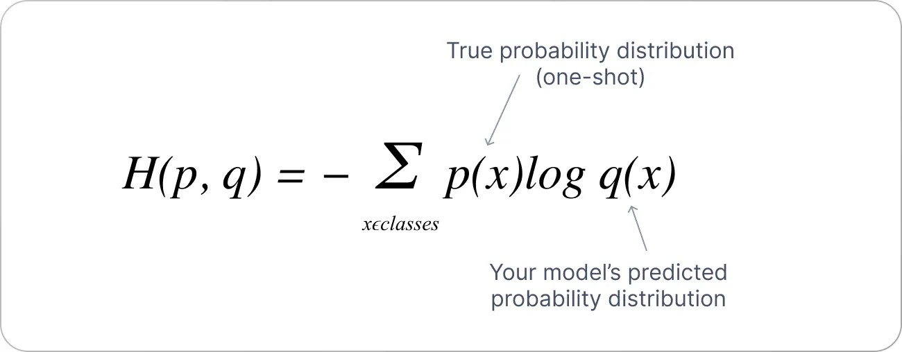 Figure 1: Cross Entropy loss formula. Source: V7 Go
Negative Log-Likelihood: Daily Forecast Pain
If your model assigns probability $q(x)$ to today’s weather, the pain you feel when it happens is:
\[-\log q(x)\]The model is confident and wrong? Then it’s a massive pain. Average this over many days (samples in our case) and you get cross entropy loss:
\[-\sum_x p(x) \log q(x)\]where $q$ is the predicted probability and $p$ is the true/label probability.
That’s why NLL or Cross Entropy is the loss function used in classification tasks where the output is a probability. You’re trying to estimate the real distribution $p$ with a model distribution $q$. Now we can see where the $\log$ term comes from :)
KL Divergence: Cost of a Bad Weather Model
Kullback Leibler (KL) divergence isolates the extra surprise caused by using the wrong beliefs:
\[D_{\text{KL}}(p||q) = \sum_x p(x) \log \frac{p(x)}{q(x)}\]Equivalent form:
\[D_{\text{KL}}(p||q) = H(p, q) - H(p)\]Interpretation:
How many extra bits of surprise you pay because your weather app is wrong.
It’s always non-negative and zero only when your model matches reality.
Importance Sampling: Studying Rare Storms
Suppose you want to estimate the probability of extreme storms.
Problem: they’re rare. Waiting around with uniform sampling will take forever.
Instead:
- Sample more often from storm-heavy cities (say distribution $q$)
- Correct the bias using importance weights:
Suppose you want to estimate:
\[\mu = \mathbb{E}_{x \sim p}[f(x)]\]where $f(x)$ is the number of storms in a month.
But sampling from $p$ rarely hits the events that matter, ie., actually storms happening.
Rewrite expectation using another distribution $q$:
\[\mu = \int f(x) p(x) dx\]Multiply & divide by (q(x)):
\[\mu = \int f(x) \frac{p(x)}{q(x)} q(x) dx \mu = \int f(x) w(x) q(x) dx\]Now sample from $q$:
\[\hat{\mu} = \frac{1}{N} \sum_{i=1}^N f(x_i) w(x_i)\]where
\[w(x) = \frac{p(x)}{q(x)}\]is the importance weight.
Interpretation:
- You sample from a convenient distribution $q$
- and then “fix” the bias using the ratio $p/q$.
This is how meteorology, finance, and ML handle rare-but-important events. This also leads us to Reinforcement Learning and is used in the most famous algorithm for learning agent policies called PPO (Proximal Policy Optimization).
The Big Picture
All of information theory revolves around one quantity:
\[-\log(\text{probability})\]- Self-information: surprise of one day
- Entropy: expected surprise
- Cross entropy: surprise under wrong beliefs
- NLL: empirical cross entropy
- KL divergence: penalty for being wrong
- Importance sampling: reweighting surprise
Information is not abstract.
It’s the mathematics of how shocked you are when reality happens.
And now you know. Fin.