HNSW - Finding Needles in Vector Haystacks

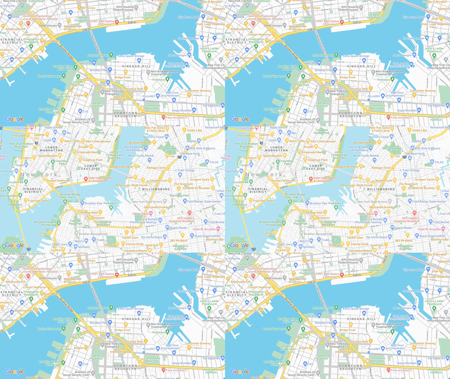
On the cover: HNSW graph depiction. Credits; https://www.marqo.ai/blog/understanding-recall-in-hnsw-search

Imagine a city with 10 million coffee shops. You (the customer) have a very specific taste vector: medium roast, cozy seating, quiet music. Now how do you go about finding the best coffee shop?

Brute Force: Visiting Every Shop

Exact Nearest Neighbor (NN) search means:

\[x^* = \arg\min_{x \in X} d(q, x)\]

where $d(q,x)$ measures “taste distance” between your shop preference $q$ and each shop $x$.

But brute force means walking into all 10 million shops to check their menu. You’d need more caffeine than your body can handle.

Approximate Nearest Neighbor (ANN): Asking for Directions

Instead of checking every café, you’re happy with one that’s “close enough.”

Formally, ANN guarantees:

\[d(q, \tilde{x}) \leq (1+\epsilon) \, d(q, x^*)\]

This is like stopping at a random coffee shops and asking the barista: “Hey, do you know a place like this?” They point you in a good-enough direction. Faster, and your latte doesn’t get cold.

Graphs: Shops That Know Each Other

Here’s the trick: connect shops into a graph.

• Nodes = coffee shops.
• Edges = friendships (two shops know each other if they’re similar enough).

Now, finding your shop means:

1. Start at some random café.
2. Ask it: “Which of your friends is closer to my taste?”
3. Walk there, repeat.

This is way better than blind wandering.

HNSW: Networking With Layers

HNSW (Hierarchical Navigable Small World) makes the city multi-layered:

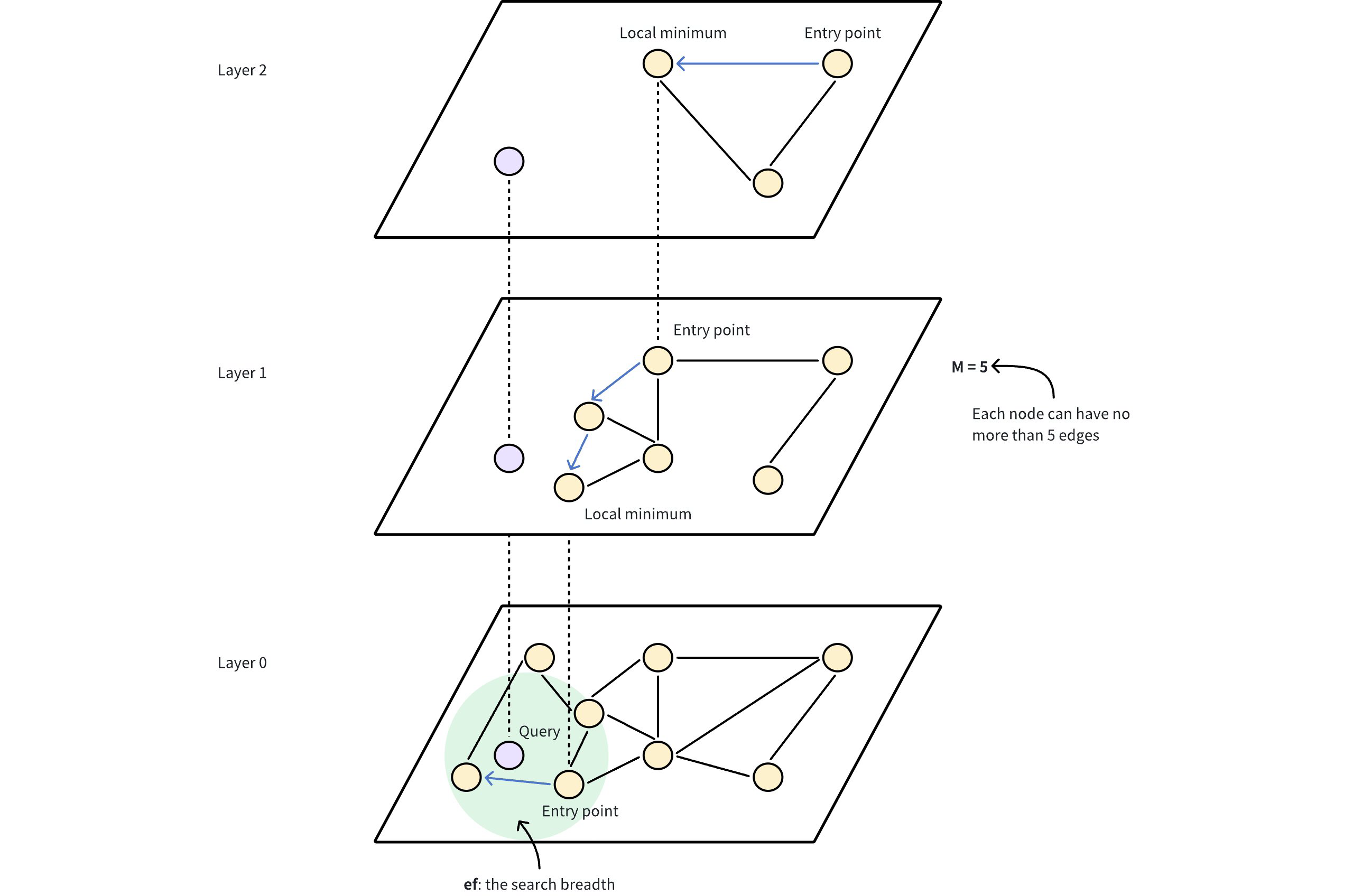
• Layer 0: The street-level café friendships (dense and local).
• Higher layers: Sparse networks where only a few cafés live — the “famous” ones, like landmark coffee houses everyone knows.
• Top layer: Just a handful (often one) “super-networked café” that acts as the entry point.

When a new shop opens, it randomly decides how high it reaches in the hierarchy. Most are only in layer 0, but some lucky cafés also make it into higher networking circles. They “live” in all the lower layers too. In expectation, the tallest “friendship ladder” is about $\log n$ layers.

Figure 1: Zooming on a city map, showing more details

Figure 2: HNSW graph as shown in Milvus

Building the Network (Construction)

When a café (node) joins the city:

1. Roll the dice to pick its maximum layer $L$. Higher levels are rare.
2. Greedy walk down: from the top landmark café, navigate layer by layer until reaching level $L$.

3. Make friends:

   • At each layer $\leq L$, search for candidate neighbors using efConstruction.
   • Keep the best $M$ matches as friends.
   • Connections are mutual — if A knows B, B knows A.

efConstruction = how aggressively a new café networks.

• Small: a quiet shop only tells a few nearby friends.
• Large: a social café hands out flyers across the city, building a rich friend circle.
• Bigger efConstruction = slower to build, but better connected graph (higher recall later).

Currently we say “a node randomly gets assigned a max layer $L(v)$.” Let’s formalize:

Each new node $v$ samples a maximum layer level $L(v)$ from an exponential distribution:

\[P(L(v) \geq \ell) = p^\ell, \quad \ell = 0,1,2,\dots\]

where $p \in (0,1)$ is a parameter (usually $p = 1/e$).

👉 This means:

• Most nodes live only in Layer 0.
• Fewer nodes appear in Layer 1, 2, …
• Very rarely, a node reaches the top layer, acting as a hub.

That’s why the top layer usually has just 1–2 nodes.

Finding Your Café (Search)

For a query taste $q$:

1. Start at the top café (the most famous one).
2. Greedy descent: at each higher layer, walk through friendships until you can’t find a closer café. Then drop one level down to that same cafe.

3. At layer 0: switch gears from greedy to exploratory search.

   • Maintain a list of candidate cafés (priority queue).
   • Size of this list = efSearch.
   • Repeatedly expand the closest candidate’s friends and update the list.
   • Stop when no closer friends are found.
   • Return the best match.

efSearch = how picky the customer is.

• Small: you settle quickly, fast search but risk missing the hidden gem.
• Large: you’re more thorough, higher recall but more steps.

Mathematically:

• Time ~ $O(efSearch \cdot \log n)$ compared to $O(N)$ for brute force.
• As efSearch grows, recall approaches 1 (exact NN), but latency grows too.

The Tuning Knobs

• M = max number of friends per café.
• efConstruction = how much effort each café puts into networking at build time.
• efSearch = how patient the customer is when asking around at query time.

Together, these decide the speed/accuracy tradeoff.

Conclusion

Brute force NN, visiting every café in town, is honest but slow. ANN is a flat graph where you’re asking for nearby cafes until you stumble upon the right spot. HNSW? It’s where you build a multi-layer city map, sprinkle in shortcuts, and then end up at the right coffee shop — almost every time.

That’s why HNSW is the backbone of modern vector databases like Milvus, Weaviate, Pinecone, Vespa. When embeddings look for their “nearest neighbor café,” they don’t wander — they network.

So the next time your vector database finds your nearest neighbor in milliseconds, remember: there’s a tiny greedy traveler sprinting down a small-world graph to make it happen.