On the cover: A Nuclear Bomb Explosion
Recently I watched this video by Veritasium talking about Markov Chains. I really liked the examples he used to explain the usage of Markov Chains, ranging from Nuclear Bombs to Google Search and Perplexity scores of LLMs. At first, comparing an Atom Bomb to Google Search might sound like the setup to a terrible joke-but in fact, they do share this wonderful mathematical lineage called Markov Chains.
In the Manhattan Project, Stanislaw Ulam and John von Neumann used them to model neutron behavior in nuclear fission; Google’s PageRank models web navigation similarly-except with links instead of neutrons and a slightly friendlier ending. But what the video lacked is perhaps a detailed mathematical explanation of how PageRank works or the math behind Perplexity scores of LLMs. In this blog, I will try to explain the math behind PageRank and Perplexity scores of LLMs.
Nuclear Bomb or Reactor: The Math Behind the Manhattan Project
Picture this: a free neutron enters Uranium-235, triggers fission, and releases more neutrons-which may in turn trigger more fissions. This cascade is inherently Markovian: each step only depends on the current generation of neutrons, not the past ones.
![]() Figure 1: Nuclear Reaction States. Source: Veritasium
Figure 1: Nuclear Reaction States. Source: Veritasium
1. The States & Transitions
Let’s simplify the system into two states:
- State A – Travelling Neutron: A neutron is free to strike a nucleus.
- State B – Leave or Absorbed: The neutron is either absorbed or escapes.
- State C - Fission: The neutron causes fission and releases more neutrons.
From State A, there are three possible transitions:
| From → To | Probability |
|---|---|
| A → A (scattered) | $p_s$: neutron scatters and continues its journey |
| A → B (absorbed or escape) | $p_a$: neutron is absorbed or escapes |
| A → C (fission) | $p_f$: neutron causes fission and releases more neutrons |
This forms a branching Markov process, since each neutron independently transitions and can spawn new neutrons or end.
2. The Math: Tracking Neutron Generations
Define $Z_n$ as the number of neutrons in generation $n$. Then:
\[\mathbb{E}[Z_{n+1} \mid Z_n] = k \cdot Z_n\]where $k$ is the average number of new neutrons produced per neutron (i.e., expected offspring).
This leads directly to the neutron multiplication factor $k$:
\[k = \frac{\mathbb{E}[Z_{n+1}]}{\mathbb{E}[Z_n]}\]- If $k > 1$: supercritical - the chain amplifies (like a bomb).
- If $k = 1$: critical - the reaction sustains itself (like in a controlled reactor)
- If $k < 1$: subcritical - the chain fizzles out.
3. Why It Matters (and Feels Like Markov Magic)
- Each neutron’s journey depends only on its current fate-completely ignoring where it came from.
- The whole system behaves like a stochastic branching process, essentially a Markov chain.
- Fission modeling via this Markovian approach was crucial in the development of nuclear reactors and weapons
PageRank: Google’s Markovian Math in Action
Let me take you deeper into the maze - starting from “random surfer” intuition, moving to matrices, and reaching the heart of the algorithm with Eigen Values that you can actually sink your teeth into.
1. The Random Surfer & Markov Chains
- Basic idea: Picture a “random surfer” on the internet. They click random links, but occasionally get bored and teleport to a completely new page.
- Markovian nature: The next page they choose depends only on what page they’re currently on-not their surfing history.
This is the essence of a discrete-time Markov chain-the same mathematical idea behind modeling neutrons in a fission process, but now repurposed for web pages. Google PageRank is a Markov Chain where the random surfer is a robot that surfs the web and the web pages are the states of the Markov Chain. The random surfer surfs the web by clicking on links and occasionally teleporting to a random page.
2. Building the Google Matrix (a.k.a. G)
-
Adjacency Matrix: Start with an adjacency matrix $A$ where $A_{ij} = 1$ if page j links to page i.
-
Stochastic Matrix: Convert it into a Markov (column-stochastic) matrix $S$ by dividing each column by the total outgoing links $k_j$. That means,
where $k_j$ is the number of outgoing links from page $j$.
- Google Matrix: For “dangling pages” (with no outgoing links), use teleportation. That means every entry in that column is replaced with $1/N$, ensuring no dead ends. This is done by using the identity matrix $I$ and scaling it by $(1-\alpha)/N$. Essentially,
where $\alpha$ is the damping factor (usually $0.85$).
Find a worked out example below to make this concrete.
3. The Stationary Distribution: $\pi = G\pi$
The goal is to find the stationary distribution $\pi$, a probability vector satisfying:
\[\pi = G \pi, \quad \sum_i \pi_i = 1\]Here,
- $\pi$ is an eigenvector of $G$.
- The corresponding eigenvalue is $1$.
Why? Because stochastic matrices always have eigenvalue $1$ (since probabilities are preserved).
We also require:
\[\sum_i \pi_i = 1, \quad \pi_i \geq 0\]This ensures $\pi$ is a valid probability distribution.
So PageRank = the unique eigenvector of $G$ associated with eigenvalue 1, normalized so entries sum to 1.
- By the Perron–Frobenius theorem, because $G$ is positive, there exists a unique, positive $\pi$.
- Intuition: over time, the random surfer visits different pages according to probabilities in $\pi$. Pages with higher $\pi_i$ are more important.
4. Power Iteration: Getting $\pi$ in Practice
Rather than solving $(I - G)\pi = 0$ directly, PageRank uses power iteration:
- Start with any initial distribution $\pi^{(0)}$ (e.g., uniform).
-
Iterate:
\[\pi^{(t+1)} = G\,\pi^{(t)}\] - Repeat until $\pi^{(t+1)} \approx \pi^{(t)}$.
This converges to $\pi$ efficiently-even in massive graphs-thanks to the matrix’s sparsity and structure.
5. Worked-Out Mini Example
Let’s a simple 3 webpage example. Assuming these are the links present in these pages:
- A → {B, C}
- B → {C}
- C → {A}
We’ll start with the adjacency matrix $A$ and stochastic matrix $S$.
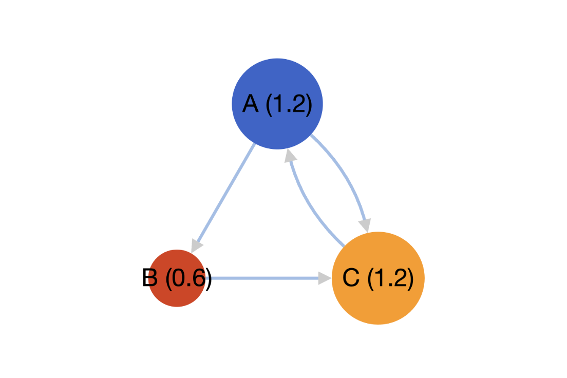 Figure 2: Webpage links illustration with $\pi$ scores after 1000 Power Iterations. Source: PageRank Simulator
Adjacency $A$ (column $j$ = links from page $j$)
\[A= \begin{bmatrix} 0 & 0 & 1\\ 1 & 0 & 0\\ 1 & 1 & 0 \end{bmatrix}\]Here, $A_{ij} = 1$ if page j links to page i.
How do we convert this into a stochastic matrix?
Now, column $j$ might have multiple 1’s (outgoing links). To turn them into probabilities:
\[S_{ij} = \frac{A_{ij}}{k_j}\]where $k_j$ = number of outgoing links from page $j$.
- From Page A: 2 links (to B and C). So each link has probability $1/2$.
- From Page B: 1 link (to C). So probability = 1.
- From Page C: 1 link (to A). So probability = 1. Outdegrees: $k_A=2,\ k_B=1,\ k_C=1$.
Column-stochastic $S$ (divide each column by its outdegree $k_j$)
So $S$ becomes:
\[S= \begin{bmatrix} 0 & 0 & 1\\ \frac12 & 0 & 0\\ \frac12 & 1 & 0 \end{bmatrix}\]Columns of $S$ sum to 1; this is the Markov transition matrix for link-following.
Google matrix $G$ with damping $\alpha=0.85$
-
Define the Google matrix:
\[G_{ij} = \alpha S_{ij} + (1 - \alpha) \frac{1}{N} I_{ij}\]where $\alpha$ is the damping factor and $I_{ij}$ is the identity matrix.
-
This means: with probability $\alpha$, follow an outgoing link; with probability $1-\alpha$, teleport to a random page.
Since $(1-\alpha)/N=0.15/3=0.05$,
\[G= \begin{bmatrix} 0.05 & 0.05 & 0.90\\ 0.475& 0.05 & 0.05\\ 0.475& 0.90 & 0.05 \end{bmatrix}.\]The $\alpha$ “teleportation” makes $G$ primitive/aperiodic so PageRank is unique and power iteration converges.
Power iteration
Start from uniform $\pi^{(0)}=(1/3,1/3,1/3)$ and iterate $\pi^{(t+1)}=G\,\pi^{(t)}$:
\[\begin{aligned} \pi^{(1)}&\approx (0.3333,\ 0.1917,\ 0.4750)\\ \pi^{(2)}&\approx (0.4538,\ 0.1917,\ 0.3546)\\ \pi^{(3)}&\approx (0.3514,\ 0.2428,\ 0.4058)\\ \vdots\ & \\ \pi^\ast&\approx (0.3878,\ 0.2148,\ 0.3974) \end{aligned}\]So C ≳ A » B in importance for this tiny graph. We can rank pages by descending $\pi_i$-there’s your “Who gets to sit at the top of search results” math.
6. Common Doubt
If there are a lot of pages pointing to a webpage, wouldn’t it automatically become the most important?
Not always. The quality, relevance, and structure of those links are just as critical-if not more.
Google’s former Search Advocate, John Mueller, emphasized:
“The total number of inbound links pointing to a website is completely irrelevant to search rankings… We try to understand what is relevant for a website… and the total number essentially is completely irrelevant. … One high-quality link from a reputable site is often far more valuable than a thousand from lower-quality sources.”
For page $i$:
\[\text{PR}(i) \;=\; \frac{1-d}{N} \;+\; d \sum_{j \to i} \frac{\text{PR}(j)}{\text{outdeg}(j)}\]where
- $d$ is the damping factor (usually $0.85$),
- $N$ is total pages,
- the sum runs over pages $j$ that link to $i$.
Read in words: PageRank of a page = a baseline teleport probability + a weighted sum of the PageRanks of pages that point to it. Each inbound link contributes $\text{PR(source)}/\text{outdeg(source)}$. So you can’t create a million dummy links and make it point to your website to increase it’s PageRank :p
SEO gurus have tried this already… And it doesn’t work.
7. Why Does It Matter?
- Relevance vs. Importance: PageRank gives a global, query-independent notion of “authority.” But when you search, Google blends this with relevance signals - keyword match, recency, personalization, and a secret sauce of hundreds of other features. Think of PageRank as the backbone; the muscles and nerves come later.
- A Family Tree of PageRanks: Over the years, Google has spun PageRank into many flavors - topic-sensitive, personalized, and who knows, maybe even a secret “cat videos only” edition. The underlying Markov principle, though, stays the same: random walks reveal hidden structure.
If the Manhattan Project mathematicians once thought tracking neutrons was tricky, they never met a billion web surfers with ADHD and a mouse.
N-Gram Models: The Word-Level Markov Chains
And just as PageRank uses Markov chains to model how a surfer hops across web pages, language models use the very same idea to predict how a word hops to the next - welcome to the world of n-grams.
If PageRank is Markov chains in the wild on the web, then n-gram models are Markov chains living in your text-predicting the next word based on the last few. It’s like your phone finishing your sentences… and often getting it wrong. Damn you, autocorrect!
1. The N-Gram Formula
In an n-gram model, to predict the probability of a word $w_i$, we approximate:
\[P(w_i \mid w_1, \dots, w_{i-1}) \approx P(w_i \mid w_{i-n+1}, \dots, w_{i-1})\]-
this is the Markov assumption in action, limiting context to the last $n-1$ words.
- Bigram (2-gram): Looks at just the previous word - e.g., $P(\text{“dog”} \mid \text{“the”})$
- Trigram (3-gram): Considers the last two words - e.g., $P(\text{“park”} \mid \text{“the”, “big”})$
2. Estimating Probabilities
We estimate probabilities using raw counts:
\[P(w_i \mid \text{history}) = \frac{\text{Count}(\text{history}, w_i)}{\text{Count}(\text{history})}\]E.g., in a bigram model:
\[P(\text{"rain"} \mid \text{"heavy"}) = \frac{\text{Count}(\text{"heavy rain"})}{\text{Count}(\text{"heavy"})}\]This is how autocorrect decides on ‘peanut butter and jelly’ instead of ‘peanut butter and belly.’
3. Handling Data Sparsity: Katz Back-off
Real-world text is messy. That means many n-grams never occur in your training data. Enter Katz’s back-off model, a neat way to handle this:
\[P_{bo}(w_i \mid \text{history}) = \begin{cases} \text{(MLE estimate)} & \text{if count > threshold} \\ \alpha \times P_{bo}(w_i \mid \text{shorter history}) & \text{otherwise} \end{cases}\]This way, if “heavy fluffy rain” never appears in your data, you back off to “fluffy rain,” and if that’s missing-back to “rain.”
Perplexity: How Confused Is the Model?
First, a quick disclaimer: we’re not talking about the startup Perplexity AI here - we’re talking about the classic perplexity score in language modeling.
So your model can generate text-but how good is it? Enter perplexity, the metric that literally asks, “Just how perplexed are you, model?”
1. What Does Perplexity Measure?
Perplexity quantifies a model’s uncertainty in predicting text. Formally:
\[\mathrm{Perplexity}(W) = \exp\left(-\frac{1}{N}\sum_{i=1}^N \log P(w_i \mid \text{context})\right)\]Or equivalently, it’s the median branching factor-how many choices the model is considering on average for the next word.
2. Perplexity in Practice
- Low perplexity: The model is confident and smooth - like your barista handing you your usual before you even order.
- High perplexity: The model is lost - like debating whether you meant *“Java” the island, *“Java” the coffee, or *“JavaScript” the language.
Perplexity is still used today to evaluate both n-gram models and large language models (LLMs). For instance, an old-school trigram model on the Brown corpus had a perplexity around 247 per word - meaning the model was basically choosing between 247 equally likely words at each step. Modern LLMs? They’ve brought this number way down, often into the tens.
| Model Type | Typical Perplexity | Insight |
|---|---|---|
| Unigram (n=1) | Very high (e.g., 900+) | No context: every word is a shot in the dark |
| Bigram | Lower (e.g., 170) | Can use the last word to narrow down guesses |
| Trigram | Even lower (e.g., 109) | More context, much less “surprised” |
| LLMs today | Often < 20 | They “see” entire paragraphs, not just 2–3 words, so uncertainty plummets |
3. Perplexity: Not Perfect, But Useful
Perplexity doesn’t tell us if the model truly understands - it only tells us how well the model predicts the next word on average. A model can be confidently wrong (like autocorrect insisting you meant “duck” :p).
Still, perplexity is:
- Grounded in entropy – measures how surprised the model is.
- Easy to compute – great for tracking progress during training.
- Still alive in the LLM era – researchers and engineers watch perplexity curves to diagnose models, even if end-user metrics (fluency, factuality) matter more in production.
Perplexity, is like a sly critic in the background: “Nice prediction - but could you sound a little less confused next time?”
Conclusion
From neutrons bouncing inside a nuclear bomb to surfers hopping between web pages, and from words tumbling out in autocomplete to entire paragraphs spun by LLMs, Markov chains are the quiet thread running through it all.
- In PageRank, they turned the chaos of the early web into an ordered map of authority.
- In n-gram models, they gave us a way to guess the next word with only a short memory.
- In perplexity, they still remind us how “surprised” our models are - whether it’s a trigram from the ’90s or GPT-5 today.
Markov chains don’t claim to understand meaning; they just keep track of what comes next. But sometimes, that’s enough. From bombs to browsers to bots, Markov chains prove that sometimes the future really is just a matter of probability. If history shows anything, it’s this: give a Markov chain enough steps, and it’ll change the world.
Fin.