On the cover: A bunch of different robots who are expert at different tasks
It’s been 8 years since the landmark paper “Attention is all you need” was published. The paper introduced the attention mechanism, which has revolutionized the field of natural language processing. The self-attention mechanism and consequently the transformer models are the main reason we have large launguage models (LLMs) today.
But these have gone through significant improvements over the years. These include the introduction of KV caching, multi-head attentions (MHA), rotary positional encodings (RoPE), and mixture of experts (MoE). In my previous post I spoke about RoPE. In this post I’ll talk about Mixture of Experts (MoE).
Intuition
Imagine one musician being asked to play every instrument in an orchestra: violin, drums, flute, trumpet, piano, even the tuba. They’d spend more time switching instruments than making music and the result would sound… questionable.
Real orchestras don’t work like that. They rely on specialized players for everything, say violinists for texture, percussionists for rhythm, brass section for power, woodwinds for color, etc. Each group is exceptional at its own style of sound. And at the center stands the conductor, who decides which section should play when, how loudly, and in what combination. They don’t need every musician for every moment, only the ones best suited for that specific passage.
This is exactly how Mixture of Experts (MoE) works. Instead of forcing a single giant neural network to handle everything math reasoning, casual conversation, coding, emotional tone, long-context reasoning, MoE creates multiple specialized sub-networks called experts. For every incoming token, a gating function acts like the conductor: it evaluates the “melody” of the input and decides which experts should play their part.
NOTE: The ability of individual experts is not exactly as depicted above. We’ll see in a later section that the experts specialize in dealing with certain types of words or phrases, for example some experts are good at learning articles whereas others are good at prepositions. A collection of experts will be needed for high level expertise such as coding or summarizing.
When transformers first appeared, scaling was simple: More layers. More width. More parameters. But this quickly hit practical limits:
- Memory limits - A 1T-parameter dense model is… unpleasant.
- Compute limits - Every forward pass activates every parameter.
- Inefficient specialisation - A single monolithic network must learn everything, even skills it rarely uses.
MoE solves this by decoupling capacity from compute. It lets you build a model with hundreds of billions or trillions of parameters, while only activating a tiny fraction (say 1–10%) for each token. This makes training faster, inference cheaper, and the architecture more modular.
Just like an orchestra creating a richer, more dynamic performance, MoE models deliver stronger results by letting the right specialists play at the right time. Mathematically, it’s concise and a little mischievous:
\[y = \sum_{i=1}^{N} g_i(x) \cdot E_i(x)\]Where:
- $(E_i(x))$ is the $(i)$-th expert.
- $(g_i(x))$ is the gating function: which expert “gets the package.”
- $(y)$ is the final output-the delivered prediction.
And the clever trick is most experts stay idle most of the time, saving compute while keeping the model huge in capacity.
Sparse MoE:
The earliest MoE proposal was dense, as in, all experts produce an output, and the gating function blends them. This was the idea from an old paper (1991) from Hinton’s reseach group in Toronto called Adaptive Mixture of Experts. The gating function is essentially a softmax that yields probabilities for each expert. Mathematically,
\[g_i(x) = \frac{\exp(f_i(x))}{\sum_{j=1}^{N} \exp(f_j(x))}\]Where:
- $(f_i(x))$ is the $(i)$-th expert.
- $(g_i(x))$ is the gating function: which expert “gets the package.”
- $(y)$ is the final output-the delivered prediction.
This works, but it computes every expert anyway, even if the gate assigns it near-zero weight. So it has zero computational savings. Dense MoE improves representation power, but not efficiency. So modern LLMs rarely use it. In the context of LLMs, Hinton and his group (a different one with Google Brain this time), released a paper called Outrageously Large Neural Networks: The Sparsely-Gated Mixture-of-Experts Layer.
The insight was simple, only activate the best K experts for each token. Instead of running all N experts: the gating function scores experts for each token, selects the top-1 or top-2 experts (top-K routing), and only those experts run. Essentially using an argmax over the softmax.
Suddenly, you get the following benefits:
- Speed - far fewer floating-point operations
- Scale - larger total capacity without larger per-token cost
- Specialisation - experts discover structure in data
- Parallelism - experts can live on different GPUs
 Figure 1: Sparse MoE architecture. Source: Outrageously Large Neural Networks: The Sparsely-Gated Mixture-of-Experts Layer
This is okay, but how do we actually apply the MoE mechanism in LLMs? Well, we apply it to the feed-forward layers of the encoder/decoder blocks. This leads to the largest savings in terms of the model compute.
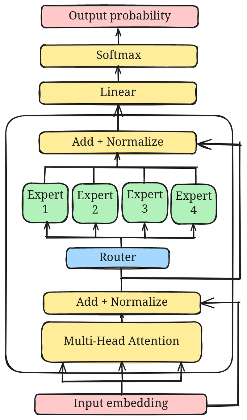 Figure 1: Sparse MoE in LLMs. Source: Dev Community
Sparse MoE is the core of Switch Transformers, DeepSeek V2/V3, GLaM, Mixtral 8×22B, and almost every modern giant model. But there’s a big danger with sparse MoE which is called router collapse.
Router Collapse
The gate/router may learn to favor just a few experts and send most tokens to them. That leaves other experts underused, defeating the purpose of having many experts in the first place. Over time, the heavily used experts get better (more data), and the underused ones stagnate, creating a vicious feedback loop.
This leads to inefficient specialization, where you don’t get the full expressive power of all experts. Another problem is load imbalance in a distributed setup (GPUs or devices). Essentially, some experts may become bottlenecks, hurting parallelism and compute efficiency.
To solve router collapse and ensure all experts contribute, the Google brain paper proposes that we use at least 2 experts (Top-2 routing), so that the model can learn to compare and use all experts. There are papers that tackle this issue in different ways. Let’s look at some of them here:
- Noisy routing
- Load Balancing with Auxiliary Losses
- Expert Capacity
- Shared experts
- Bias based loss-free Load Balancing
1. Noisy Routing
The first trick comes straight from the original sparsely-gated MoE paper: add noise to the router logits. Instead of picking experts based purely on the model’s confidence, we add a Gaussian noise term:
\[\tilde{z}_i = f_i(x) + \epsilon,\quad \epsilon \sim \mathcal{N}(0,\sigma^2)\]This forces occasional exploration. Even if the router strongly prefers Expert 3 today, a bit of noise nudges it to check what Expert 7 has been up to lately. Over time, this prevents early lock-in and encourages experts to discover meaningful specializations.
Think of it as the router saying: “Sure, violin section is great… but maybe let’s see what the clarinets can do for this musical phrase.”
2. Load Balancing with Auxiliary Losses
This is the classic technique introduced in the GShard and Switch Transformer papers.
This loss encourages all experts to receive roughly equal numbers of tokens and encourages the router’s attention distribution to stay balanced. Mathematically,
-
Average gate probability (also called importance score or mean gate): \(P_i = \frac{1}{T}\sum_{t=1}^T p_{t,i}\)
-
Empirical fraction of tokens dispatched (the load): \(f_i = \frac{1}{T}\sum_{t=1}^T \mathbb{I}[\mathrm{assign}_t = i]\)
The loss is then computed as: \(\mathcal{L}_{balance} = \lambda \cdot E \cdot \sum_{i=1}^{E} P_i , f_i\)
Where (\lambda) is a small hyperparameter (loss weight).
This loss look like tiny penalties during training, but they play the role of the orchestra conductor whispering: “Hey, brass section, stop overpowering everyone; give the flutes a chance.”
The downside? You’ve now added extra gradients, hyperparameters, and another term that must be tuned. But for many early MoE models, this was the most effective stabilization method.
3. Expert Capacity (Capacity Factor)
Every expert gets a maximum number of tokens per batch. If an expert is at capacity, the router must pick someone else-even if that expert has the highest score.
Formally, each expert can only accept:
\[C = \text{capacity factor} \times \frac{T}{E}\]where
- (T) = tokens in the batch
- (E) = number of experts
This prevents “expert hogging.” Switch Transformers famously rely on this and simply drop excess tokens when capacity is exceeded (a bit brutal, but surprisingly works).
DeepSpeed-MoE and GLaM use more graceful spillover techniques, where the next-best expert is chosen instead.
This is a loss-free method-no extra optimization needed.
4. Shared Experts (Dense + Sparse Hybrid)
Modern models like Mixtral 8×22B discovered a neat trick: combine a small shared dense feed-forward layer with a larger sparse MoE layer.
Every token always goes through the shared FFN, and then the sparse experts provide additional specialized processing. This stabilizes training because:
- gradients always flow through a shared path
- router mistakes are less catastrophic
- underused experts matter less early on
You get the stability of dense models with the efficiency of MoE-a best-of-both-worlds design.
5. Bias-Based Load Balancing (Loss-Free)
This is one of the more modern and elegant approaches from DeepSpeed-MoE. The idea is beautifully simple:
- Track how often each expert is used.
- If an expert is overused → add a small negative bias to its logit.
- If an expert is underused → add a small positive bias.
Mathematically:
\[\tilde{z}_i = f_i(x) + b_i\]with bias ($b_i$) updated based on usage statistics. No extra loss function. No tuning of balance weights. No additional backprop.
This encourages the router to “spread the love” without interfering with the main optimization objective. This technique is smooth, adaptive, and almost invisible unlike loss-based methods.
Big Picture
Dense models are hitting diminishing returns. Training a model 2× larger no longer gives you 2× improvements and the cost is enormous.
MoE flips that equation: You can scale parameters without scaling compute.
This is why almost every frontier model roadmap includes MoE variants. For the next several years, MoEs will likely be the central scaling strategy for large language models, just like attention was from 2017-2023.
MoE is not just a “research idea.” It’s becoming the production-grade architecture for trillion-parameter intelligence.
And now you know. Fin.