RoPE - Is Attention All You Really Need?

On the cover: A RoPE, essentially

It’s been 8 years since the landmark paper “Attention is all you need” was published. The paper introduced the attention mechanism, which has revolutionized the field of natural language processing. The self-attention mechanism and consequently the transformer models are the main reason we have large launguage models (LLMs) today.

But these have gone through significant improvements over the years. These include the introduction of multi-head attentions (MHA), rotary positional encodings (RoPE), mixture of experts (MoE), and KV caching. In my previous post I spoke about MLA and KV caching. In this post I’ll talk about Rotary Positional Encodings (RoPE).

Going Round in Circles: From Naive to RoPE

Transformers (GPT, BERT, etc.) process tokens in parallel, so they have no built‑in sense of word order. To give them “where in the sentence” information, we add positional encodings to each token embedding. This is important because transformers don’t have any sense of word order.

Think of it this way - if you just toss all your word embeddings into a blender, the transformer has no idea who did what to whom. Without positional info, “the cat ate the mouse” and “the mouse ate the cat” look identical. Same words, same embeddings, just… mixed up. Positional encodings are like giving each word a little GPS tag saying, “Hey, I’m the 1st word!” or “I’m the 5th one, hanging out near the end.”

Integer, One-Hot and Binary Encodings: A Bumpy Beginning

Naively, you could tag each token with its integer index $(0,1,2,…)$. But that runs into problems – treating position as a raw number can bias the model. It might think “position 7 > position 3” means more important.

What about one-hot position vector $(\mathbf{1}_{p})$ where $p$ is the position index? Here all positions are zero except for the index position which is 1. But this runs into problems as well - one-hot vectors can grow large and they don’t generalize beyond the max length seen in training.

What about binary encoding? The binary encoding refers to converting the position index into binary (e.g. position 5 → binary $101$). It’s compact, but it’s highly discontinuous. Adjacent positions can flip multiple bits, causing big jumps in the encoding space. For example, going from position 3 (binary $011$) to 4 (binary $100$) flips all bits, which is a huge “distance” in encoding even though tokens moved just one step.

In a learning model we want small changes in position to produce small changes in encoding, so the model can interpolate and learn patterns across positions. Binary is more like a staircase: jagged and hard to generalize, especially to positions beyond those seen in training. Essentially binary does give us one-hot-style schemes with unique codes, but they’re so discontinuous that the model struggles to grasp smooth positional relationships.

We essentially need a representation that is unique for each position but also smooth in the way it changes from one token to the next. How can we achieve this? Binary doesn’t cut it for us. But there are patterns in binary encoding, that lead to a better encoding model.

Consider these binary encodings assuming 8-bit representation, $PE_{p,i}$ where $p$ is the position index and $i$ is the index of the binary encoding ($i \in {0,1,2,3,4,5,6,7}$). This can be seen below:

\[PE_{0,0:8} = 00000000\\ PE_{1,0:8} = 00000001\\ PE_{2,0:8} = 00000010\\ PE_{3,0:8} = 00000011\\ PE_{4,0:8} = 00000100\\ PE_{5,0:8} = 00000101\\ PE_{6,0:8} = 00000110\\ PE_{7,0:8} = 00000111\\ PE_{8,0:8} = 00001000\\ PE_{9,0:8} = 00001001\\ PE_{10,0:8} = 00001010\\ PE_{11,0:8} = 00001011\\ ...\\\]

What we can see is that the lowest bit (i.e. $PE_{p,0}$) varies a lot compared to the higher indices (i.e. $PE_{p,7}$). This is intentional. Because the immediately closer words need to be distinguished. Whereas the higher indices vary less frequently and can capture the long term relationships. A visual might help; I made a plot of the binary encodings for positions 0 to 120 with 8 dimensions.

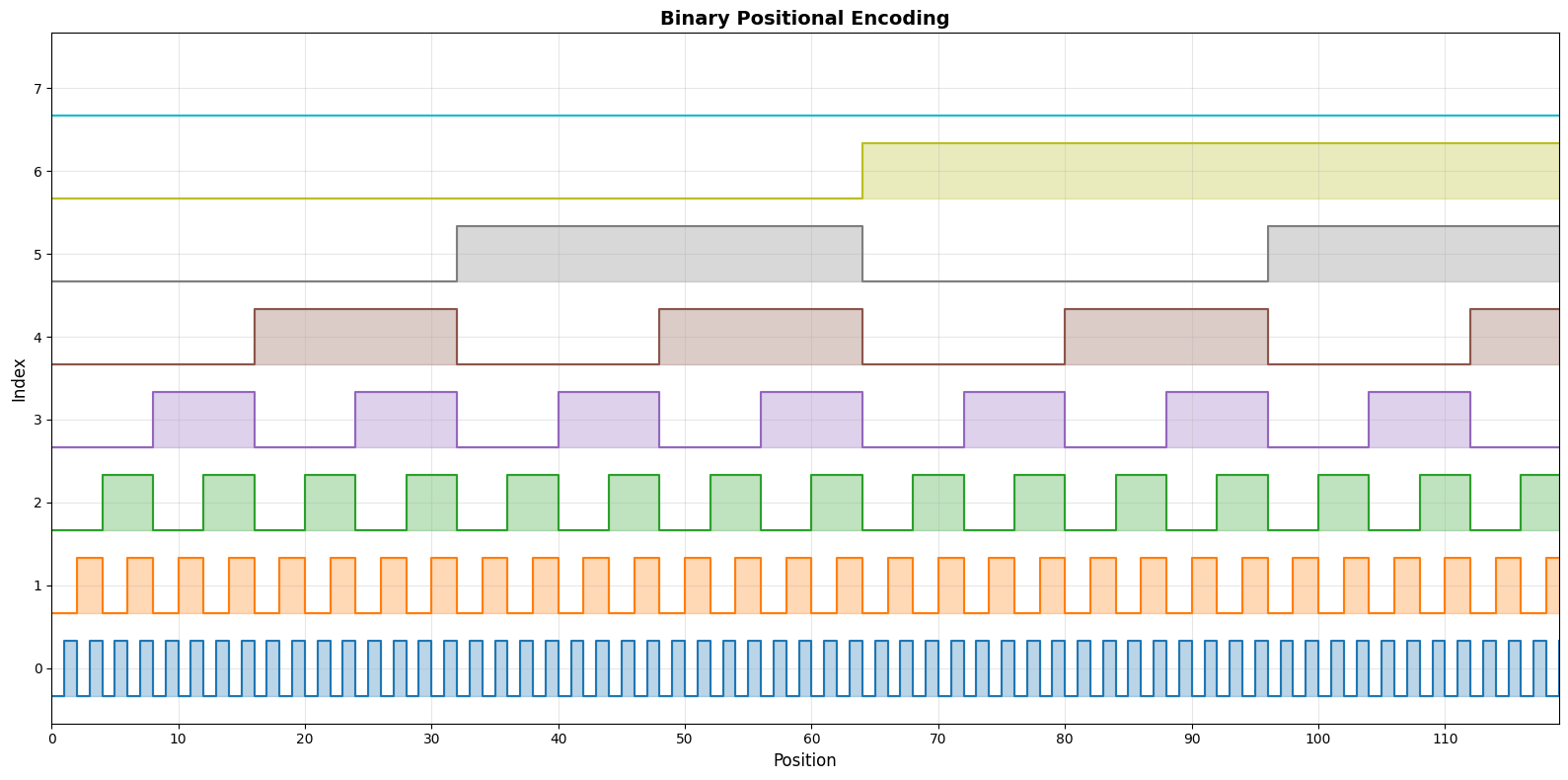alt Figure 1: Binary Encoding of sequential integers. Source: Author

The above plot shows the periodicity of the indices which helps in extrapolating to longer sequences. But one needs to increase the number of dimensions to capture the periodicity. This becomes a problem as the number of dimensions are usually fixed during training.

The plot also shows that the binary encoding is highly discontinuous with a step function and the model struggles to learn smooth positional relationships. To address the problem of discontinuity we can approximate it using a smooth function like sine and cosine. This is exactly what the authors did in the paper “Attention Is All You Need”.

Sinusoidal Encodings: Riding the Waves

The sinusoidal encodings introduced in the paper “Attention Is All You Need” are a smoother alternative to binary encodings. Each position is encoded by a vector of sine and cosine values at different frequencies at different indices (of d-dimensions). Concretely, for a token at position $p$ in a $d$-dimensional model and index $i$, they set:

\[PE_{p,2i} = \sin\bigl(\tfrac{p}{10000^{2i/d}}\bigr)\\ PE_{p,2i+1} = \cos\bigl(\tfrac{p}{10000^{2i/d}}\bigr)\\\]

so that each even dimension is a sine wave and each odd dimension is a cosine wave of a different wavelength. The wavelengths form a geometric progression (from $2\pi$ up to $10000 \cdot 2\pi$), ensuring each position gets a unique multi-frequency “signature.” Because sine and cosine are continuous, the encoding changes smoothly as $p$ increments, satisfying the desire for small position shifts to cause small encoding shifts.

Everyone who’s read the paper has seen these out of place equations at the end of the architecture. On first glance it sort of makes sense, but not really. So we take it for granted and assume that it all works. A quick plot shows the sinusoidal encodings for positions 0 to 120 with 8 dimensions.

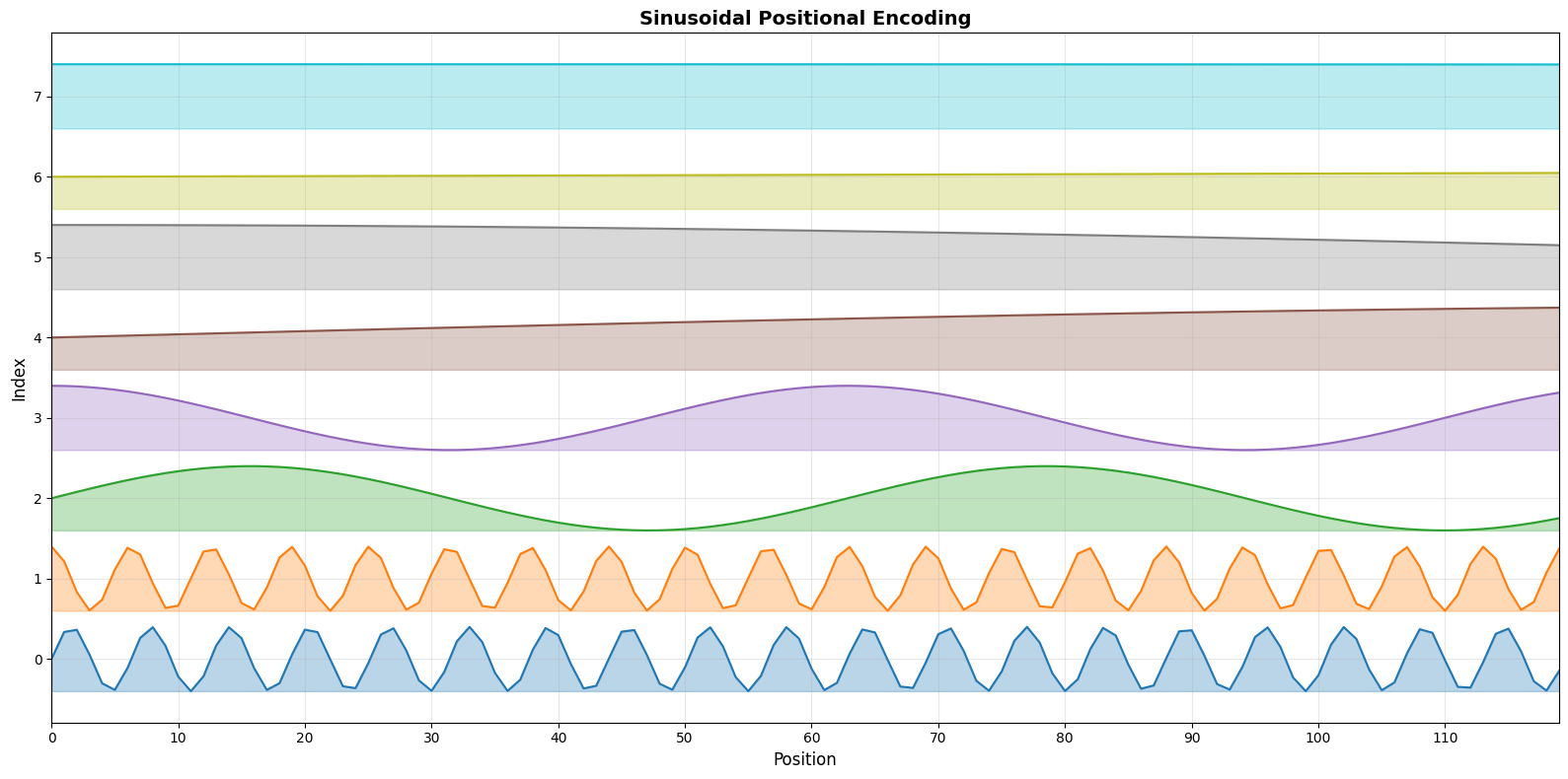alt Figure 1: Sinusoidal Encoding of sequential integers. Source: Author

Doesn’t this look extremely similar to the binary encodings except smoother? But there are a couple of questions:

Why use sine and cosine for even and odd indices of the vector?
Why use a frequency $\omega_i = 10000^{2i/d}$?

Sine and Cosine

This choice makes relative positions easy to learn. The Transformer authors pointed out that shifting a sine/cosine position by a fixed offset is just a linear transform of the encoding, i.e. $PE_{p+k}$ can be expressed as a linear function of $PE_p$ for pairwise indices of the positional embedding vector.

\[PE_{p+k} = \begin{bmatrix} \cos(k\theta_1) & -\sin(k\theta_1) \\ \sin(k\theta_1) & \cos(k\theta_1) \end{bmatrix} PE_p\]

In other words, the network can attend “by relative positions” without extra hassle. Also, because these are fixed functions (not learned vectors), the model can extrapolate beyond the training length. Indeed, Vaswani et al. noted that learned vs. sinusoidal encodings gave similar results, but favored sinusoids because “they may allow the model to extrapolate to sequence lengths longer than those seen in training.” Intuitively, you can think of each position sliding along a fixed multidimensional sine wave – even if you go further out than in training, the pattern keeps repeating in a controlled way.

Frequency Term

Now, about that mysterious $10000^{2i/d}$ term in the denominator, it’s not random math magic. Each embedding dimension corresponds to a different frequency of sine and cosine. Smaller indices wiggle fast to capture local order (“who’s next to whom”), while larger indices change slowly to capture global position (“am I near the start or end?”).

The exponential term $10000^{2i/d}$ spreads these frequencies out in a geometric progression, giving the model both fine and coarse positional detail — like tuning each dimension to a different radio wavelength. Why Geometric Progression (GP)? Why not Arithmetic Progression (AP)? Well, you need a large range of varying frequencies to capture the positional information. And AP is too slow for this.

And the 10,000? Arbitrary. It just keeps the slowest waves slow enough for typical sequence lengths. In short: $10000^{2i/d}$ gives sinusoidal encodings their multi-scale rhythm — smooth, unique, and easy for the model to learn from.

Keeping Track of Distance: Why Relative Position Matters

Even with sinusoidal encodings, later work observed that relative distance between tokens often matters more than their absolute positions. For example, models like Transformer-XL and T5 introduced explicit bias terms based on $|m - n|$ — because words two apart should interact differently than words fifty apart.

Sinusoidal encodings do allow the model to infer these relations indirectly (thanks to their linear shift property), but they mix positional and semantic information through addition — the position vector gets added to the token embedding. This changes the direction of the embedding and slightly warps its meaning.

Rotary Positional Embeddings (RoPE) fix that by applying position as a rotation in embedding space instead of an addition. Each token’s representation is rotated by an angle proportional to its position, so relative offsets become explicitly encoded in the dot product between tokens. In short:

Sinusoidal PE → add position → semantics slightly change, relative distance encoded indirectly

Rotary PE → rotate position → semantics preserved, relative distance encoded directly

Rotary Positional Embeddings (RoPE): The Twist

RoPE takes a simple but powerful approach: instead of adding positional information to token embeddings, it rotates the query and key vectors after they’ve been projected through their weight matrices. That means the token’s semantic meaning (the embedding itself) stays intact — position is only introduced when the model is about to compute attention.

Formally, for a token at position $p$:

\[\mathbf{q}_p = \mathbf{x_p W_Q} \\ \mathbf{k}_p = \mathbf{x_p W_K} \\\]

and then RoPE applies a position-dependent rotation matrix $\mathbf{R}(p)$:

\[\mathbf{q^\prime}_p = \mathbf{R}(p)\mathbf{q}_p \\ \mathbf{k^\prime}_p = \mathbf{R}(p)\mathbf{k}_p \\\]

Concretely, we split each $d$-dimensional vector into 2D sub-vectors and rotate each pair. For example, for the $i$th 2D pair we do:

\[\begin{bmatrix} q'*{2i} \\ q'*{2i+1} \end{bmatrix} = \begin{bmatrix} \cos(m \theta_i) & -\sin(m \theta_i) \\ \sin(m \theta_i) & \cos(m \theta_i) \end{bmatrix} \begin{bmatrix} q_{2i} \\ q_{2i+1} \end{bmatrix}\]

and similarly for $k$. Here $\theta_i$ is a base angle for that subspace (often chosen like $\theta_i=10000^{-2i/d}$, matching the sinusoidal frequencies).

Why rotate? The magnitude is preserved, so no semantic information loss unlike the sinusoidal encoding.

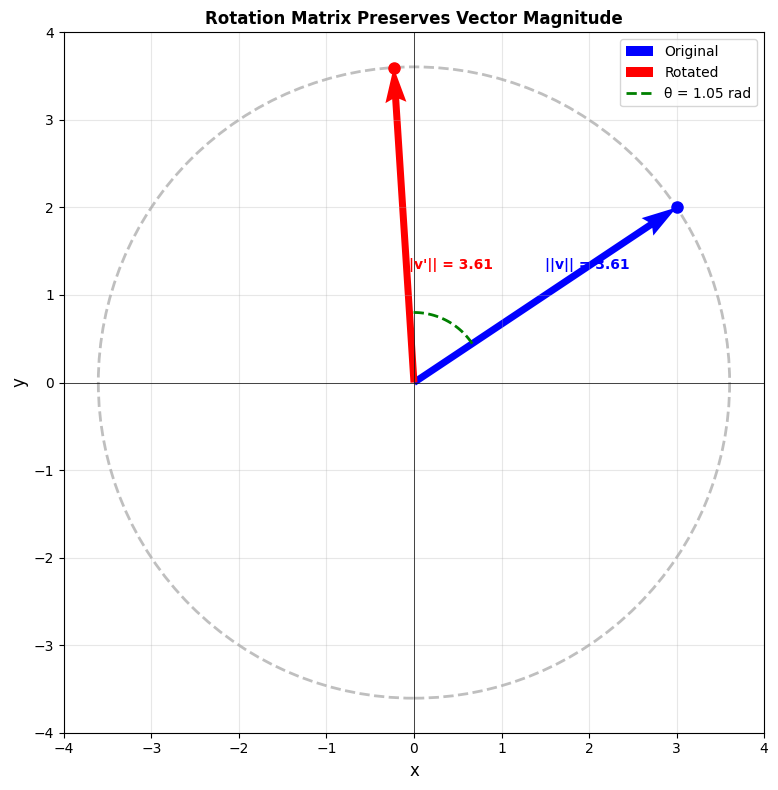alt Figure 2: Vector Rotation preserved magnitude. Source: Author

One more nice thing about this is that the dot-product of rotated vectors injects relative position. After rotation, the attention score between position $m$ and $n$ becomes:

\[\mathbf{q}_m^\top \mathbf{k}_n = \mathbf{q}_m^\top \mathbf{R}(m)^\top \mathbf{R}(n) \mathbf{k}_n\]

Notice that $\mathbf{R}(m)^\top\mathbf{R}(n)$ is just a rotation by $(n-m)\theta$. In other words, the dot product depends only on the difference $(n-m)$, i.e. the relative offset. This elegantly bakes relative distance into self-attention. As the original RoFormer paper puts it, “simply rotate the word embedding vector by an amount of angle multiple of its position index” to incorporate relative position.

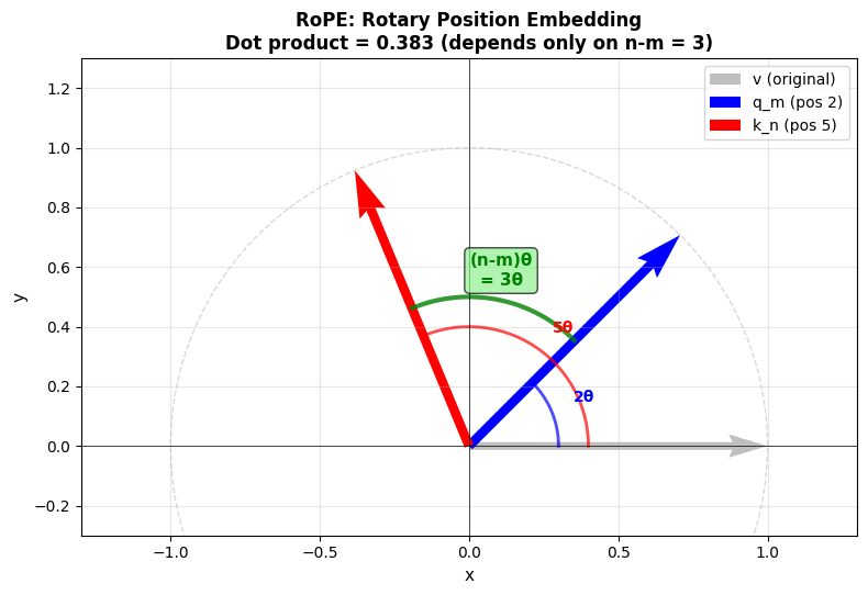alt Figure 3: Rotary Position Embedding in action. The query vector (blue) at position $m$ is rotated by an angle $m\theta$ say $2\theta$, and the key vector (red) at position $n$ by $n\theta$ say $5\theta$. After rotation, their inner product depends on the difference $(n-m)$ say $(5-2)\theta = 3\theta$, so attention is a function of token distance rather than their absolute positions.Source: Author

\[\mathbf{R}(m)^\top \mathbf{R}(n) = \mathbf{R}(n-m)\]

meaning the combined effect is a rotation by $(n-m)\theta$. Plugging into the attention score:

\[{\mathbf{q}'_m}^\top \mathbf{k}'_n = \mathbf{q}_m^\top \mathbf{R}(m)^\top \mathbf{R}(n)\,\mathbf{k}_n = \mathbf{q}_m^\top \mathbf{R}(n-m)\,\mathbf{k}_n\]

Thus the interaction only “sees” the distance $(n-m)$. In effect, RoPE transforms absolute encodings into relative ones through rotation. Importantly, rotation matrices are orthonormal (they preserve vector length), so RoPE doesn’t distort the embedding norms – it’s a clean, stable transform.

Why RoPE Rocks: Benefits and Intuition

Rotary encoding packs many nice properties into a simple idea:

Absolute+Relative in One: By rotating each token’s Q/K by its own position, RoPE implicitly encodes both “where is this token?” (absolute) and “how far from another?” (relative). This dual nature comes for free.
Flexible Sequence Length: Like the sinusoidal case, RoPE is not learned per index so you can run it on arbitrarily long sequences. There’s no fixed maximum position cap.
Distance Decay: The choice of angles (often matching the sinusoid scaling) means that as (n-m) grows, the effective dot product tends to “mix” more of both sin and cos components, causing a gradual decay. In fact, the RoFormer paper proves that the attention scores naturally shrink as distance increases, aligning with the intuition that very distant tokens should connect less strongly.
Linear-Attention Friendly: Because rotation preserves norms, RoPE works seamlessly even in linear-time attention mechanisms (e.g. Performers). In contrast, many relative-encoding schemes require adding bias terms or adjustments that don’t play nicely with kernelized attention. RoPE’s multiplicative, orthogonal nature means it can be plugged into any self-attention variant without extra tricks.
No Extra Parameters: There are no new learned embeddings – just (fixed) sinusoidal angles. It’s purely a geometric trick on the existing Q/K vectors, so it adds almost no overhead.
Empirically Strong: In practice, RoPE has proven effective. The RoFormer paper reports consistent gains over baselines on long-text benchmarks. Hugging Face even notes that RoPE “allows a model to track absolute positions and model relative relationships” and that it “can scale to longer sequences, account for decay of token dependencies, and works with efficient linear self-attention”.

In short, RoPE gives you a rotational highway to encode “where” each token is while letting their interactions depend on “how far apart” they are. The result is a cleaner, theoretically-motivated positional scheme that plays well with modern Transformer variants.

So essentially we now have a better modeling of long sequences and easier learning of positional patterns – all with a clever bit of trigonometry.

And now you know.

Fin.