On the cover: Midjourney’s creation for the prompt “Astronauts exploring an alien red planet”
Diffusion models are all the rage these days. Why do we need these new models for image generation? In fact, we have GANs, VAEs and Flow models that have had sucess before. If you consider text-to-image generation, there are versions such as StackGAN, AttnGAN and VQ-VAE. But recently, diffusion models have taken the center-stage because of their high quality, high diversity and high fidelity (compliance to text prompts). Some of the popular diffusion models that has hit the news are:
- DALL-E2 (OpenAI)
- Imagen (Google Brain)
- Midjourney (independent company)
- Stable diffusion (StabilityAI)
Why did diffusion models take-off only now? I would say that GANs (2014) and VAEs (2013) had a head-start and were practically useful since their inception (pun-intended). The theory of diffusion models as a neural network have been around since 2015. It’s only recently (2020-21) that the tricks required to make it run practically such as modifying the objective to predicting noise, variational lower bound for variance, faster sampling using implicit models, classifier free guidance, etc. were introduced.
In this two part blog post, we will take a look at the physical intiution, training and sampling of diffusion models, followed by the various guidance aspects. I’ve brushed past most of the derivations and loss function formulations for the sake of brevity and clarity in explanation. Please refer to the original papers if you’re keen on them.
Physical intuition
Diffusion is a well-defined physical process. Consider an ink droplet in a glass of water: it starts off with a unique shape (complex density distribution) when first dropped and it mixes down to the shapeless uniformity of water (uniform distribution). So we can think about diffusion as a process, where the structure of a substance get destroyed sequentially in time leading to just noise.
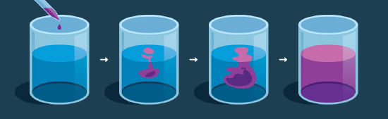 Figure 1: Diffusion of ink droplet in a glass of water
It is mathematically easy to represent the final uniform distribution, but much harder to represent the initial complex density distribution. Oookay, is it possible to start with the easy final distribution and arrive at the harder initial distribution? Well, the physical process of diffusion is spontaneous and irreversible (meaning you cannot unbreak a glass; please don’t try at home).
However, it is possible to model this irreversible process through a neural network. And we can learn the initial density distribution as well! How do we do that you ask? Well we can make use of this nice observation from the diffusion process: when you look at the ink droplet in water microscopically and for a small time period, the forward and reverse processes look exactly the same! If I ask you whether the short clip below of diffusion is forward in time or backwards, I bet that your guess is as good as a coin flip. We will make use of this nice property in our neural network.
 Figure 2: Brownian motion of particles in diffusion. Forwards and reverse in time is indistinguishable
What’s underneath?
- During the forward diffusion process $q$, we take a good image $x_0$, destroy and add noise to it sequentially little by little to get an isotropic gaussian noise image $x_T$ ($t=0,1,2,…,T$). Here isotropic means that it looks same in all directions (mathematically, $\boldsymbol{\Sigma} = \sigma^2 \boldsymbol{I}$)
- During the reverse diffusion process $p_\theta$ we use a neural network to transform from noise $x_T$ back to the original image $x_0$, sequentially
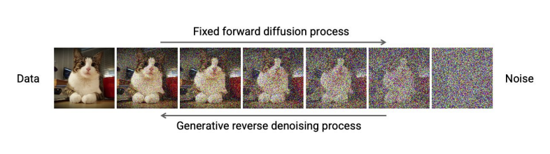
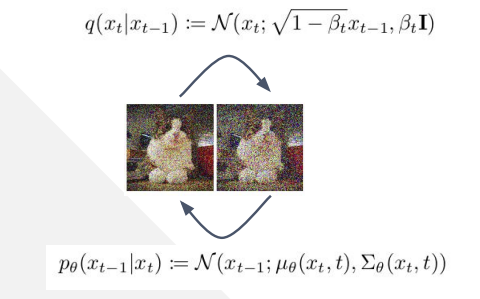 Figure 3: Forward and reverse diffusion processes.
We can see that in the forward diffusion, each successive image is sampled from a Gaussian distribution which is dependent on the previous image and noise (information destruction and noise addition). Since we know that the forward and reverse process look the same under micro conditions, we can model the reverse diffusion by a Gaussian as well! How neat. The mean and variance of this reverse Gaussian distribution is obtained by transforming the input image $x_t$ by a neural network with learnable parameters $\theta$. Why Gaussian though? Why not Uniform, Laplace, Poisson or other distributions? That’s because Gaussian noise is quite common in imaging systems. Also, in these equations below, ${\beta_t \in (0,1) }^T_{t=1}$ is diffusion scheduling parameter that determines how much noise is added and how much destruction is happening.
Tricks
There are couple of tricks to make the training and sampling of these models easier. Some of these are as follows:
-
To get to a random timestep, need not sample repeatedly, use reparameterization. Essentially you can rewrite the noise scheduling parameter as follows: $\alpha_t = 1-\beta_t$ and $\bar{\alpha_t} = \prod_{s=0}^t \alpha_s$. This makes the forward diffusion $q(x_t \vert x_0) = \mathcal{N}(x_t; \sqrt{\bar{\alpha_t}} x_0, (1 - \bar{\alpha_t}) \boldsymbol{I})$
-
One can have various schedules for the diffusion parameter $\alpha_t$. Improved DDPM suggest using cosine-scheduling which provides near-linear drop in the middle of the training process and subtle changes around t=0 and t=T which we can see in the figures below. $\quad\bar{\alpha_t} = \frac{f(t)}{f(0)}\quad\text{where }f(t)=\cos\Big(\frac{t/3T+s}{1+s}\cdot\frac{\pi}{2}\Big)^2$
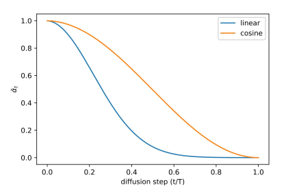
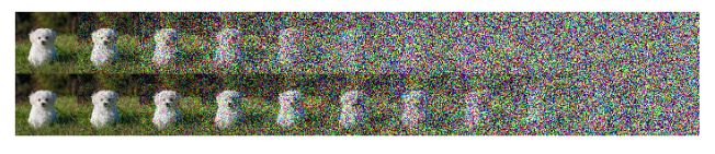 Figure 4: Beta schedule comparison for linear and cosine schedule
 -
Predict the noise instead of the mean directly; they are equivalent. From the DDPM paper, “We have shown that the $\epsilon$-prediction parameterization both resembles Langevin dynamics and simplifies the diffusion model variational bound to an objective that resembles denoising score matching”. The relation between $\mu_\theta(x_t, t)$ and $\epsilon_\theta(x_t, t)$ is given as, $\mu_\theta(x_t, t) = \frac{1}{\sqrt{\alpha_t}} \Big(x_t - \frac{1 - \alpha_t}{\sqrt{1 - \bar{\alpha_t}}} \epsilon_\theta(x_t, t) \Big)$. Thus images can be sampled as follows by using the predicted noise: $x_{t-1} = \mathcal{N}(x_{t-1}; \frac{1}{\sqrt{\alpha_t}} \Big(x_t - \frac{1 - \alpha_t}{\sqrt{1 - \bar{\alpha_t}}} \epsilon_\theta(x_t, t) \Big), \Sigma_\theta(x_t, t))$
-
Variance can be either fixed or learned; learned variance reduces number of timesteps during sampling. Improved DDPM propose to have a learned variance as follows by the model predicting a mixing vector $\mathbf{v}$: $\Sigma_\theta(x_t, t) = \exp(\mathbf{v} \log \beta_t + (1-\mathbf{v}) \log \tilde{\beta_t})$ where $\tilde{\beta_t} = \frac{1 - \bar{\alpha_{t-1}}}{1 - \bar{\alpha_t}} \cdot \beta_t$
Training and Sampling
Training
- Take an image $x_0$, sample $t \sim [1,T]$, destroy and add noise $\epsilon \sim \mathcal{N}(0,\boldsymbol{I})$ to it through the schedule $\alpha_t$ to get image $x_t$
- Train a model $\epsilon_\theta(x_t, t)$ (with say a U-Net architecture) given inputs of noisy image xt and timestep t, predicts the noise that was added
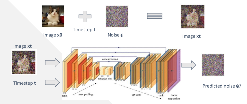 Figure 5: Training process depiction
Sampling
- Start with random noise $x_T \sim \mathcal{N}(0,\boldsymbol{I})$ and use the model $\epsilon_\theta(x_t, t)$ to predict the noise
- Convert the predicted noise $\epsilon_\theta(x_t, t)$ to mean $\mu_\theta(x_t, t)$
- Sample the previous image $x_{t-1}$ from the distribution $p_\theta(x_{t-1} \vert x_t) = \mathcal{N}(x_{t-1}; \mu_\theta(x_t, t), \Sigma_\theta(x_t, t))$
- Repeat from $t=T$ till $t=0$
- In practice however, instead of sampling from the distribution $p_\theta(x_{t-1} \vert x_t)$, we compute the $x_0 = \frac{1}{\sqrt{\alpha_t}} \Big(x_t - \frac{1 - \alpha_t}{\sqrt{1 - \bar{\alpha_t}}} \epsilon_\theta(x_t, t) \Big)$ and add a noise $z \sim \mathcal{N}(0,\boldsymbol{I})$ to it to get $x_{t-1}$.
- Now you might ask, hey I already got $x_0$ here, why do I need to go and add noise and make it $x_{t-1}$ and repeat the whole thing again? The computed $x_0$ at each step is a prediction based on the current noisy input, but it isn’t perfect. Repeating the process over many steps gradually refines the image, allowing the model to correct errors incrementally rather than relying on one single leap from noise to a clean image.
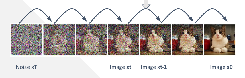 Figure 3: Sampling process depiction
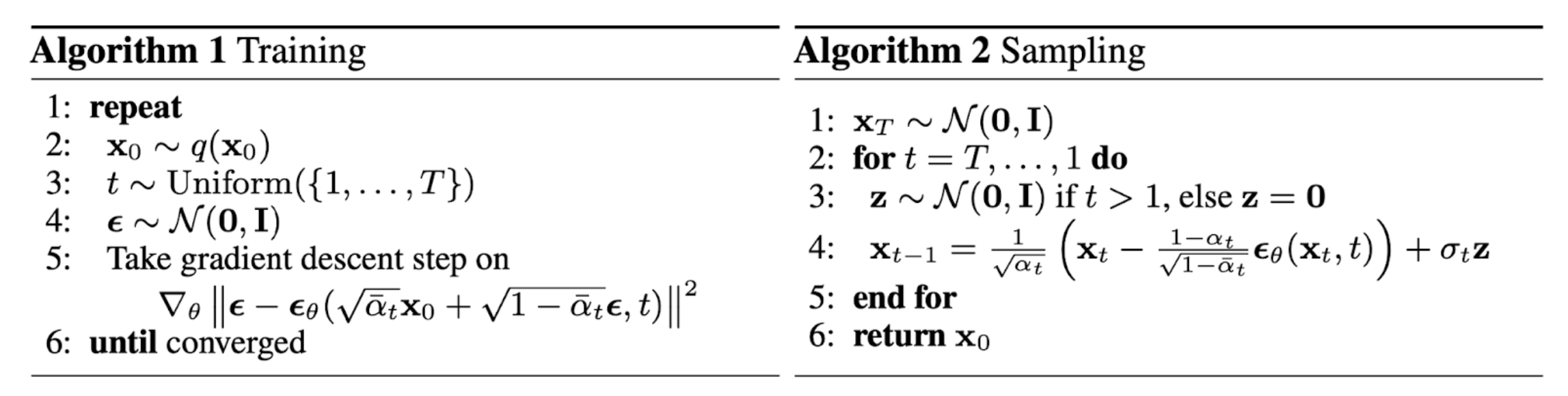 Figure 3: Training and sampling algorithms for diffusion models from DDPM
The algorithms diagram above shows this process nicely. Alright, so far we have seen how to train a diffusion model and sample from it. If we sample from this trained model it will give us random samples. How do we get the model to give us say a picture of a Cute Cat Cthulu with tentacles instead of arms? In the next post we will look at guidance for diffusion models to achieve this. Stay tuned! :)
 Figure 3: Cute Cat Cthulu generated from Midjourney