
On the cover: Stephen Bishop’s map of Mammoth Cave in Kentucky, drawn from memory in 1842 and published in 1845. Bishop was an enslaved man who worked as a guide at the cave. Public domain, via Wikimedia Commons.

In January 2016, John Tromp finished counting the legal positions on a 19 by 19 Go board: about $2.08 \times 10^{170}$, a 171-digit number. The observable universe has around $10^{80}$ atoms. Give every one of those atoms its own universe of $10^{80}$ atoms, and put one Go position on each. You would still have covered only one position in every twenty billion.
Two months later, AlphaGo beat Lee Sedol, one of the best Go players alive, 4 games to 1. It never came near looking at all those positions. Its search, Monte Carlo tree search (MCTS), looks at a tiny corner of the tree, picked by playing games out at random. This post builds MCTS from scratch and runs it on a real Go position and a real chess position. Part 2 is how AlphaGo and AlphaZero wrapped neural networks around it, and how that connects to PPO.
Why search a tree at all
A game is a tree. Every position is a node, and every legal move is a branch to the position it leads to. So picking a move means asking which branch leads to a win.
You can pick by reflex: look at the board and play what looks right. A neural network trained on expert games does this pretty well, and AlphaGo’s first network guessed the expert’s move 57% of the time. But a reflex never asks what the opponent will do next. Looking ahead does. You follow a move down the tree, assume the opponent answers with their best reply, and see where you end up. This rule is called minimax. If you could follow every line to the end of the game, it would play perfectly.
You can’t. The AlphaGo paper puts chess at about 35 legal moves per turn over about 80 moves, and Go at about 250 over about 150. That is roughly $10^{123}$ paths through the chess tree and $10^{360}$ through the Go tree.
So chess programs stop after a set number of moves and score the position with a hand-written formula (an evaluation function). It counts the material, adds a bit for king safety and takes a bit off for a doubled pawn. They also skip branches that provably cannot change the answer (alpha-beta pruning). That recipe beat Kasparov in 1997, and Stockfish, the strongest chess engine today, still uses it.
Why Monte Carlo
Go breaks that recipe, because nobody could write the formula. The rules are simple: two players take turns placing stones, a surrounded group is captured, and whoever surrounds more of the board wins. But a single stone is worth nothing by itself, and whether a group survives can depend on one point, forty moves later. Before 2006, the best Go programs played at about 14 kyu, the level of somebody a few months into a Go club.
The Monte Carlo idea is to stop trying to write the formula. If you can’t score a position, play it out. Play random moves for both sides until the game ends, note who won, and do that a few thousand times. The fraction of games your side wins is the score. (“Monte Carlo” is the usual name for anything built on random sampling, after the casino.) Random moves are terrible moves, so why does this work? Because a position where you win 70% of random games is usually better than one where you win 30%. Go suits it well: every game ends, the final count is simple, and a big lead tends to survive a lot of bad play.
Bernd Brügmann tried this on 9 by 9 Go in 1993. His program played thousands of near-random games after each candidate move and picked the best average. It reached about 25 kyu, roughly a beginner. This flat Monte Carlo has two problems. It spends as many games on bad moves as on good ones. And it assumes the opponent plays at random, so a move that loses to one precise reply still looks fine.
The fix came in 2006: put the random games in a tree. Each game adds its result to the moves it passed through. Moves that do well get more games, so the tree grows deeper along the good lines. And at the opponent’s turns, the tree assumes they pick their best reply. Kocsis and Szepesvári proved that with enough games, the chance of picking the wrong move goes to zero. Rémi Coulom built a Go program on the same idea that year, and his paper is usually credited with the name. Within a few years, Go programs went from 14 kyu to around 5 dan (a strong amateur).
| approach | how it scores a position | expects the opponent’s best reply | where it breaks |
|---|---|---|---|
| minimax to the end | plays every line out | yes | the tree is far too big |
| alpha-beta with a formula | a hand-written evaluation function | yes | Go has no formula |
| flat Monte Carlo | random games after each move | no | falls for one precise reply |
| MCTS | random games, steered by a tree | yes | sharp traps, and it starts out blind |
So when does MCTS fit? When four things are true:
- You can simulate: given a position and a move, you can work out the next position.
- There is a clear result at the end, a win, a loss or a score.
- The tree is too big to search fully, and nobody can write a good formula to score positions part way.
- You have time to run hundreds or thousands of simulated games before each decision.
Most of daily life fails the first two. There is no rulebook for replying to your landlord. And you cannot run Thursday evening eight hundred times to see which dinner went best.
The caving club
I want you to think about a wild cave that a local caving club has been mapping for twenty years, on weekends, with a tape measure. Every trip takes four people six hours (and one of them always forgets the spare batteries). Every chamber has three or four more holes leading out of it. So they will never survey the whole thing. What they have instead is a survey book, and a rule for where to go next Saturday.
A junction in the cave is a position (the state $s$), and a passage out of it is a legal move (the action $a$). For each passage the book keeps two numbers: how many trips have gone down it ($N(s,a)$, the visit count), and how well they went on average ($Q(s,a)$, the value). A won game scores 1 and a lost one scores 0. With two players, the book scores each junction’s passages for whoever is choosing there, which is minimax again.
One simulation is one trip, and it has four steps:
- Select. Walk down from the entrance through junctions already in the book, taking the passage with the best score at each.
- Expand. When you reach a junction the book has never seen, add it.
- Evaluate. Play random moves from there to the end of the game and see who wins (a rollout). Later programs ask a neural network instead.
- Back up. Walk back out, adding one to $N$ and folding the result into $Q$ for every passage you came through.
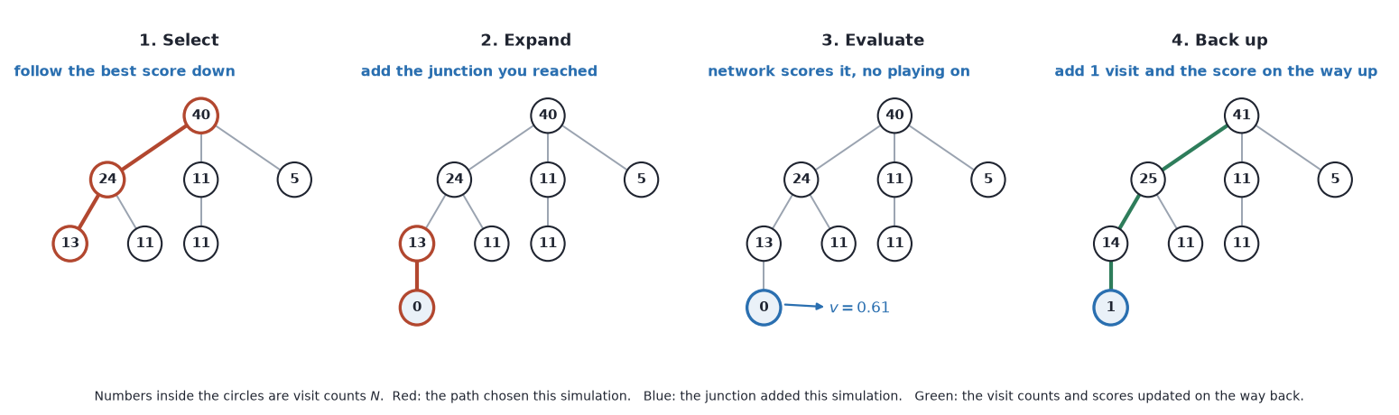 Figure 1: the four steps of one simulation. The search runs this loop hundreds of times before it plays a single move. Source: Author
Run the loop a few hundred times and the book fills up very unevenly, because the promising passages get most of the trips. When it is time to play, which passage does the club commit to? The one with the most visits. A passage with a wonderful average from two trips might just have been lucky twice. A passage with 412 trips has survived 412 chances to disappoint everybody.
Which passage next
The select step needs a scoring rule. Kocsis and Szepesvári took theirs from the maths of slot machines (the multi-armed bandit problem), and it is called UCT:
\[\text{score of a passage} = \text{how well it has gone so far} + \text{a bonus for having had few trips}\]specifically, in its usual textbook form,
\[a_t = \arg\max_a \left[\, Q(s,a) + c \sqrt{\frac{\ln \sum_b N(s,b)}{N(s,a)}} \,\right]\]where $a_t$ is the passage the trip takes, $\arg\max_a$ means “the passage that makes the bracket biggest”, $Q(s,a)$ is the average result of the trips down passage $a$, $N(s,a)$ is how many trips those were, $\sum_b N(s,b)$ is the total over all passages out of this junction, $\ln$ is the natural log, and $c$ is a constant that sets how big the bonus is (how much the club likes trying new holes).
The bonus shrinks every time a passage is walked, and slowly grows while the others are. A passage with no trips has an infinite bonus, so it gets tried first. That’s it. There is no knowledge of Go in there, only counts and averages.
Here is the whole search in Python. It is the exact code behind the two examples below:
class Node:
    def __init__(self, state, move=None, parent=None):
        self.move, self.parent, self.children = move, parent, []
        self.untried = state.legal_moves()            # moves not in the tree yet
        self.first_moved = not state.first_to_move()  # did the first player make `move`?
        self.n, self.w = 0, 0.0                       # visits, total result for that player


def uct_search(root_state, rollout, n_simulations, c=1.0, seed=0, on_step=None):
    rng = random.Random(seed)
    root = Node(root_state)
    for t in range(1, n_simulations + 1):
        node, state = root, root_state.copy()

        # 1. Select: walk down through fully expanded nodes by UCT score
        while not node.untried and node.children:
            log_n = math.log(node.n)
            node = max(node.children,
                       key=lambda ch: ch.w / ch.n + c * math.sqrt(log_n / ch.n))
            state.play(node.move)

        # 2. Expand: add one untried move to the tree
        if node.untried and not state.is_over():
            move = node.untried.pop(rng.randrange(len(node.untried)))
            state.play(move)
            child = Node(state, move, node)
            node.children.append(child)
            node = child

        # 3. Simulate: play the rest of the game out at random
        result = rollout(state, rng)

        # 4. Back up: every node on the path scores the result for its mover
        while node is not None:
            node.n += 1
            node.w += result if node.first_moved else 1 - result
            node = node.parent

        if on_step:
            on_step(t, root)
    return root


def best_move(root):
    """Play the most-visited move, not the one with the best average."""
    return max(root.children, key=lambda ch: ch.n).move
A game only has to provide five methods: copy, legal_moves, play, is_over and first_to_move. It also needs a rollout function that plays the game out and returns 1 if the first player won and 0 if they lost. The full scripts, with the Go rules and the chess setup, are on GitHub.
Plain MCTS on a Go position
Black’s group in the bottom-left corner of this 7 by 7 board has three empty points inside it: A1, B1 and C1. A group needs two separate empty points inside it (two eyes) to be safe for good. If Black plays B1, the group has two eyes, A1 and C1, and lives. If White plays B1 first, it can only ever make one eye, and dies. The rest of the board is settled, so this corner decides the game. Go players have a proverb for it: your opponent’s vital point is your vital point.
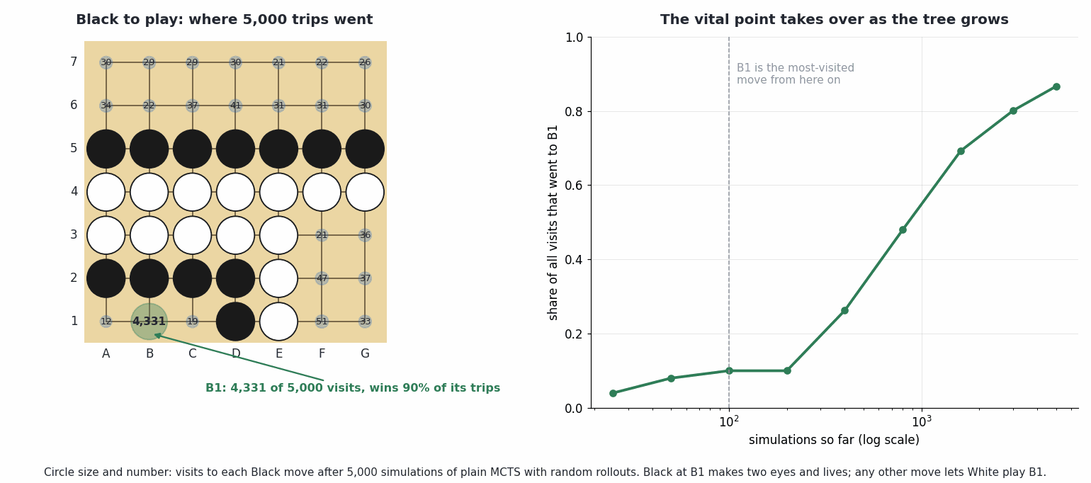 Figure 2: plain MCTS, 5,000 simulations, Black to play. Left, the visits each Black move got. Right, B1’s share of all visits as the search went on. Source: Author
After 5,000 simulations, which took about six seconds, B1 had 4,331 of the visits and won 90% of its games. The next move, F1, had 51 visits and won 53%. B1 was the most-visited move from 100 simulations on. The 90% comes from the rollouts. After B1, the group lives in every random game. After any other move, it lives only if Black happens to reach B1 before White does, which is about half the time.
Plain MCTS on a chess position
Chess is where random games go wrong. Here, White’s queen can take the knight on d7 for free. But the queen is the only piece guarding e1, and White’s own pawns box the king in. So after Qxd7, Black plays Re1 and it is mate.
I ran two searches with the same rollout: six random moves, then count the material. Flat Monte Carlo, with 400 random games after each of White’s 26 moves, scores Qxd7 best of all at 0.686, ahead of Kf1 at 0.626. A random Black reply finds Re1 one time in twenty, so most of those games just see White a knight up.
MCTS likes Qxd7 too at first, and it is the most-visited move between about 200 and 500 simulations. But each visit adds one more of Black’s replies to the tree. Once Re1 is in, it wins every trip for Black, so the search keeps choosing it. Qxd7’s average sinks with each of those trips. After 5,000 simulations Qxd7 had 73 visits. The top moves were f4, f3, Kf1, h3, g4 and h4, and none of them takes the queen off the first rank.
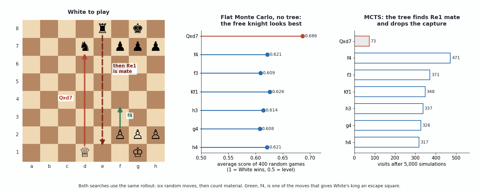 Figure 3: the same rollouts, with and without a tree. Flat Monte Carlo ranks the free knight first. MCTS gives it 73 visits out of 5,000. Source: Author
Where plain MCTS runs out
Plain MCTS took Go programs to strong amateur and stopped there. More simulations help, but they don’t fix these:
- Sharp tactics. Ramanujan, Sabharwal and Selman (2010) call them shallow traps: moves that lose to a short, forced sequence. Plain MCTS caught traps three moves deep but missed them at five and deeper. The trap above was one move deep, so the tree found it fast. Chess is full of deeper ones, which is part of why chess engines stayed with alpha-beta.
- A blind select step. UCT knows nothing about the game, so at a junction with 250 moves it has to try every one before it can prefer any.
- Noisy rollouts. Random moves are nothing like good moves. So it takes thousands of rollouts to say anything, and they can still misjudge a position a strong player reads in a second.
Conclusion
MCTS is a small idea. When you can’t score a position, play it out at random, and keep a tree of where those games went so that the next ones go somewhere useful. It needs nothing but the rules, and on a 7 by 7 board it found a vital point that Go players learn from a proverb. And a visit count is just a tally of where the club spent its Saturdays.
Part 2 gives the club a nose and a draught: AlphaGo’s policy and value networks, then AlphaGo Zero, where the search becomes the network’s teacher, and how that loop connects to PPO.
Stay tuned for Part 2. Till then ciao.