
On the cover: a page from a notation notebook. The letters sit in their beat boxes, and the red squiggles are what somebody added where the letters were not enough. The last boxes are empty because the singer was still going. Source: Author.
In the Mamba post I said that nobody feeds a Transformer raw audio samples. Speech models like Whisper, OpenAI’s speech recogniser, turn the sound into a spectrogram first. Then they squash that down to about 50 chunks a second. I called it a hand-built shortcut and moved on.
I want to come back to that shortcut, because it has a second problem that I skipped. A spectrogram is a picture, and every number in it can sit anywhere on a dial. But a language model does not predict a dial. It predicts the next item from a fixed list, the way the tokenizer kept a case of 50,257 pieces of metal type. Ask a model for the next picture and there is no list to pick from.
So here is what you get if you stop there: a model that writes down every word you said and cannot say one of them back in your voice.
Welcome to the era of audio tokens. This is the story of how a second of sound became a list of whole numbers short enough to talk with, and of what those numbers leave behind in the room.
I want you to sit through a concert with me first. It is December in Chennai, the music season, a hall with ceiling fans and four hundred plastic chairs. On stage there is a singer, a violin and a mridangam. Two people in that hall are taking the concert down. In the fifth row a student has a ruled notebook and is writing swara letters into little boxes, one to a beat: S, R, G, M, P, D, N. At the back, somebody has a tape recorder running.
By the end of the night both of them have the concert. The notebook can be read and argued over on the bus home, and it weighs nothing. The tape has every hair of the singer’s voice, and it is a mile of brown ribbon nobody can read. What this post is after is the third thing, a notebook you can sing from.
A second of sound, in numbers
Sound is air pressure going up and down. A microphone measures that pressure on a schedule, usually 16,000 or 24,000 times a second. Each measurement is one number, and a digital recording is nothing more than that list.
So one minute of talking at 24,000 measurements a second is 1,440,000 numbers. The Mamba post already priced what happens when you call each one a token: ten seconds of it fills an 80 GB H100 with the memory of somebody saying hello.
Size is only half the trouble. A model that predicts text ends in a softmax, which hands out a probability for every item on a list (the cross entropy post is the long version of that sentence). You can force samples onto a list by rounding them to 256 levels, which is what WaveNet did in 2016. It sounded good, and it needed 16,000 predictions a second.
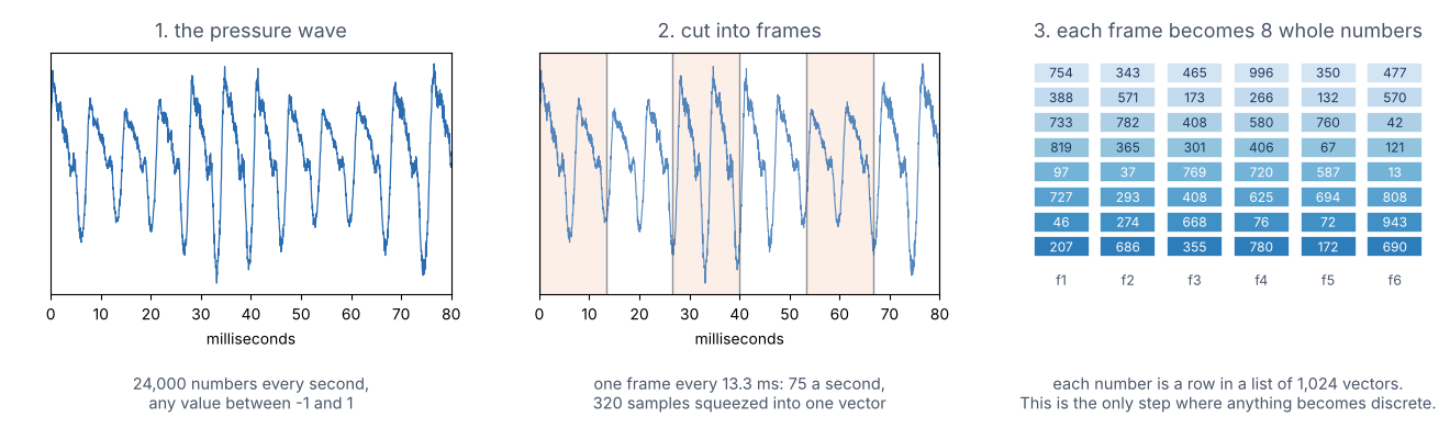 Figure 1: the pipeline in one line. Only the last step makes something a model can pick off a list. Source: Author
Two things are wanted at once, then:
- A short list of symbols a second, few enough to hold a whole conversation.
- Enough in them to rebuild a sound somebody would recognise as you.
Every method below is good at one and has to be argued into the other.
The notebook with a picture in it
The oldest trick is to stop looking at the wave and ask what is inside it. Take 25 milliseconds of audio, multiply it by a smooth window so the cut edges do not click, and ask how much energy sits at each frequency. That is one frame. Slide along by 10 milliseconds and do it again, which gives 100 frames a second (Whisper’s first convolution then halves that to the 50 I quoted above). Mathematically, each frame is a Fourier transform of a windowed slice:
\[X(m, k) = \sum_{n=0}^{N-1} x(n + mH)\, w(n)\, e^{-2\pi i k n / N}\]where $x$ is the waveform, $w$ is the 25 ms window, $N$ is its length in samples, $H$ is the 10 ms hop between frames, $m$ is which frame we are on and $k$ is which frequency bin. Each $X(m,k)$ is a complex number with a size and an angle. Keep the size, drop the angle, and you have a spectrogram.
That dropped angle is the phase, and it causes trouble later. The frequency axis then gets squashed onto the mel scale, because your ear separates two low tones far better than two high ones. So the bands are narrow down where the vowels live and wide up where the hiss is, forty of them or so:
\[\text{mel}(f) = 2595 \log_{10}\left(1 + \frac{f}{700}\right)\]Those two constants come from no theory at all. Somebody in the 1930s sat volunteers in a room and asked which tone sounded twice as high as another, and 2595 and 700 are what fell out of the curve they drew. The 700 is what keeps the scale nearly straight below a kilohertz and bends it into a log above. Every voice assistant on earth still runs on them.
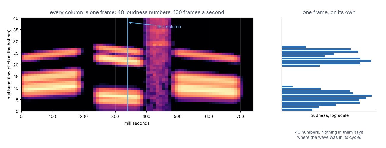 Figure 2: about 0.7 seconds of synthetic speech. The horizontal bars are vocal tract resonances; the fuzzy vertical block is a consonant. Source: Author
That picture is all a recogniser needs, and Whisper still uses it. But you cannot sing from it. The phase went in the bin, partly because it looks like noise on a plot and is miserable to model. So turning a spectrogram back into audio means inventing a phase that fits, and a vocoder is the network that does the inventing. And it is still a grid of numbers, not a list of symbols. Our student has drawn the concert, not written it.
The scribe nobody taught the letters
What if you let a model invent its own letters? Nobody handed the student the swara names on day one. He sat through a hundred concerts, noticed the shapes that keep coming back, and learnt the names.
wav2vec 2.0 does that. It runs the raw wave through a convolutional stack to get one vector every 20 milliseconds, masks out chunks of them, and makes the model pick the right one out of a line-up of fakes. The targets are quantised into two small codebooks of 320 entries each, combined, so 320 × 320 = 102,400 possible units. After pre-training on 53,000 hours of unlabelled speech, ten minutes of transcribed audio gets it to 4.8% word error rate on the clean half of LibriSpeech, a thousand hours of audiobooks read aloud. On the noisier half it manages 8.2%. Ten minutes of labels.
HuBERT, short for hidden-unit BERT, is cruder and works about as well. Run k-means on plain MFCC features, the 1980s speech descriptor, with 100 clusters, and call each cluster a letter. Mask parts of the audio and train the model to predict which letter was there. Then throw the k-means away, re-cluster the model’s own features, and go round again.
The ablation is the funny part. Those first 100 clusters are pretty bad, in that they match no phoneme a linguist would recognise. The paper’s own conclusion is that the method leans on the consistency of the clustering rather than the quality of the labels. The teacher only has to be wrong the same way every time, and the student sorts out the rest.
So these units know what was said. Ask them who said it and the answer is gone, because speaker and pitch and room got flattened out, and that flattening is what made them good at recognition. They are the letters in the boxes, without the squiggles.
One list will not do
We want symbols you can play back, which means the symbol has to carry the sound itself. So why not keep one enormous list and look the frame up in it? Let’s do the sums.
Take 24 kHz audio and an encoder that makes 75 frames a second. Say we want 6 kbps, about what a thin phone call costs. That is 80 bits a frame. If one symbol carries all 80, the list it comes from needs $2^{80}$ entries, which is about $1.2 \times 10^{24}$ vectors. At 128 numbers each, a typical encoder width, and four bytes a number, that table weighs some $6 \times 10^{14}$ terabytes. For one codec. Somebody please price the rack.
The fix is a ladder, and it is called residual vector quantisation (RVQ). Pick the nearest entry from a list of 1,024 and subtract it from the frame. What is left over is the residual. It goes to a second list of 1,024 that has learnt where the first one’s leftovers land. (Every entry is learnt during training, dragged towards the vectors that keep choosing it.) Subtract again. Do it eight times. In words:
\[\text{what is left after } k \text{ passes} = \text{the frame} - (\text{guess 1} + \text{guess 2} + \dots + \text{guess } k)\]specifically,
\[r_k = x - \sum_{j=1}^{k} c_j[i_j], \qquad i_k = \arg\min_i \Vert r_{k-1} - c_k[i]\Vert^2, \qquad r_0 = x\]where $x$ is the frame vector, $c_j[i]$ is entry $i$ of codebook $j$, $i_k$ is the index pass $k$ writes down, and $\Vert \cdot \Vert$ is ordinary distance. Eight indices of ten bits come to the same 80 bits. But what you store is 8 × 1,024 = 8,192 vectors, about 4 MB, against that $6 \times 10^{14}$ terabytes. That is the whole trick, and it costs eight nearest-neighbour searches instead of one.
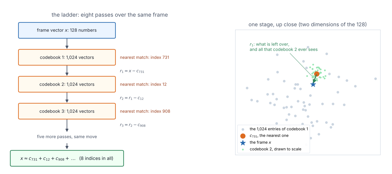 Figure 3: the ladder on the left, one rung up close on the right. Codebook 2 never sees the frame, only what codebook 1 got wrong, which is why its entries sit so much tighter. Source: Author
One note on the word, because it collides. This is not the quantisation of the quantization post, where a number went from 16 bits to 4. Here a whole vector is swapped for the nearest entry in a list.
Eight scribes in a row
SoundStream (Google, 2021) was the first to put the ladder inside a trained codec, which is short for coder-decoder. A convolutional encoder takes 24 kHz audio down by a factor of 320, so 75 frames a second. The RVQ turns each frame into indices, and a mirrored decoder turns them back into a wave. On top of the reconstruction loss sit adversarial discriminators and a multi-scale spectrogram loss. Those are what stop the output sounding like a fax machine (anyone who has heard an early vocoder knows the sound).
At 3 kbps, which is four rungs rather than eight, it beat Opus, the codec your video calls actually run on, at 12 kbps. The ladder’s length is what sets the bitrate. That is four times the compression, judged by human listeners, and it runs faster than real time on a phone.
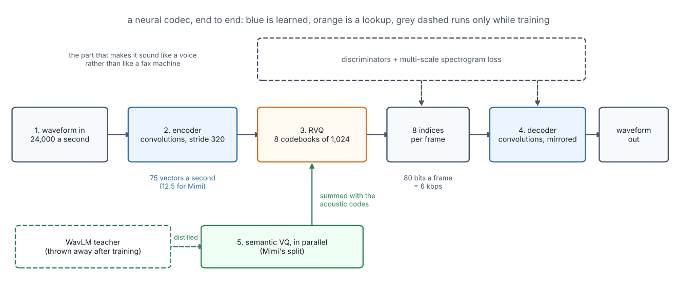 Figure 4: one codec, end to end. The dashed boxes get deleted the moment training stops, which is a poor deal for something doing that much of the work. Source: Author
EnCodec (Meta, 2022) is the same shape at the same 75 frames a second, with better training. One model covers 1.5 to 24 kbps, thanks to quantiser dropout: in training it randomly uses only the first few rungs, so those learn to stand on their own. Two codebooks is 1.5 kbps, eight is 6 kbps, all thirty-two is 24 kbps. A small Transformer then squeezes the indices by up to 40% more, still faster than real time.
What the letters know and what the squiggles know
There are two notebooks on the table now, and AudioLM (Google, 2022) said use both. Semantic tokens, from a BERT-style speech model clustered into 1,024 units at 25 a second, carry what is being said. Acoustic tokens, from a SoundStream configured here at 50 frames a second and twelve codebooks, carry the voice. AudioLM generates the semantic ones first, then coarse acoustic ones conditioned on those, then the fine detail. Eight streams are not free for a next-token model either, so Moshi runs a small second Transformer down the eight codebooks of a frame.
Why bother with the first stage? Because a model trained on acoustic tokens alone babbles. It sounds exactly like the speaker and wanders off the point, because nothing in those tokens holds a sentence together.
Voice cloning falls out of the same codes. VALL-E (Microsoft, 2023) treats text-to-speech as next-token prediction over EnCodec codes, trained on 60,000 hours of audiobooks. Give it three seconds of a stranger talking and it continues in that voice, room acoustics and all, which is either marvellous or alarming depending on the week you are having.
| Notebook | What it keeps | Can you play it back? | Symbols a second | What it is for |
|---|---|---|---|---|
| Mel spectrogram | loudness per band | only if a vocoder guesses the phase | not symbols at all | recognition |
| HuBERT units | the words, mostly | not recognisably | 50 | understanding, cheaply |
| EnCodec codes | everything, down to the room | yes, that is the design | 600 at 6 kbps | compression, cloning |
| Mimi codes | both, on purpose | yes | 100 | models that talk back |
Mimi, and the price of writing fast
Now look at that fourth column again, because for a model that has to talk, that column is the budget. It reads audio tokens and writes them into the same window text has to fit in.
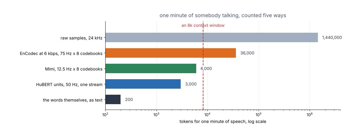 Figure 5: one minute of speech, counted five ways, against an 8,192-token context window. EnCodec at 6 kbps spends that whole window in thirteen seconds. Source: Author
Mimi, the codec inside Moshi (Kyutai, 2024), is built for that budget. It takes 24 kHz audio down to 12.5 frames a second, with 8 codebooks of 2,048 entries. That is 100 symbols a second at 11 bits each, so 1.1 kbps all in. It is causal, so it never looks ahead. One frame of latency works out to 80 milliseconds. A minute of talking costs 6,000 tokens instead of 36,000.
Dropping the rate that far means each frame carries more, so Mimi makes its first codebook carry meaning. The method is distillation: a frozen WavLM plays teacher, and the first quantiser is trained to match what WavLM thinks. Then the teacher is thrown away.
Here is the ablation, and I like it because the authors published the part that went wrong. Putting the semantic job on the first rung does improve phonetic discriminability, measured by the ABX error rate, which asks whether two sounds land on the right side of a phoneme boundary. But it hurt audio quality, because every rung below now works with a residual shaped by somebody else’s objective. So they split it: a plain semantic quantiser in parallel with a 7-level acoustic ladder, outputs summed. MUSHRA, the listening test where people score clips against a hidden reference, went from 57.8 to 64.0. ABX got worse, from 6.5% to 8.1%. They took the trade, and they printed both columns in the paper.
Today that split is what ships. Moshi and the stacks after it read and write codec tokens instead of text, VALL-E’s descendants dub films off three seconds of audio, and Whisper’s family owns everything that never has to be played back.
Where things are going
- Lower frame rates. 12.5 Hz is 80 milliseconds a frame, about the length of a short consonant. Go much below and one frame straddles two sounds.
- One model, two streams. Moshi runs a text stream beside the audio as an inner monologue, so the planning happens in words while the mouth happens in codes.
- Skipping the codebook. Diffusion and flow matching systems build audio straight from continuous vectors and never discretise. They are harder to splice into a language model, which is why the discrete route got there first.
- Codecs graded by the model, not the ear. Mimi’s distillation started it, and the next will be scored on how well a model learns from their tokens.
The gamaka problem
A gamaka is the slide and shake between notes that makes Carnatic music what it is. Write the letters down, hand them to somebody who learnt from the page, and you get the notes with none of the music. Every complaint below is a version of that gap between the page and the room.
Nobody agrees what a good notebook sounds like. MUSHRA needs a room of humans in headphones, so it is slow and pricey. ABX and word error rate are cheap and measure other things. Mimi’s own table has the two moving in opposite directions, so a leaderboard here is won by picking which column to print.
The words semantic and acoustic are aspirational too. They say which end of the ladder a thing came from, not what it carries. HuBERT units keep more speaker identity than “semantic” suggests, and a codec’s first rung picks up phonetics by itself.
Then there is the data, almost all of it English, read aloud, in a quiet room: LibriSpeech and Libri-Light are audiobooks. A tonal language where pitch changes the word, an ornamented singing style, two people code-switching mid-sentence, a call taken on a scooter: none of it is in there in any quantity. A codec fitted on read English has no reason to spend bits on a pitch slide, so the gamaka is an engineering problem, not only a nice image.
And 12.5 Hz is a budget decision in a lab coat. It is where the token count stopped embarrassing the language model, and the quality numbers came back tolerable. That is a fine way to build something, though it says nothing about the natural rate of speech.
My sourcing is uneven as well. arXiv and Wikimedia are both blocked from the machine I write these on, so the links here are for you rather than for me. So the SoundStream, EnCodec and Mimi internals come from abstracts and secondary write-ups rather than the figures. The bitrate arithmetic checks out against the published rates, which is why I trust it. The number I would most like checked is Mimi’s 2,048-entry codebook, which I derived from the bitrate rather than read.
Conclusion
A microphone gives you 24,000 numbers a second and no way to say any of them. Turn those into a spectrogram and a recogniser can read it, but nobody can sing from it. Let a model invent its own letters and you get the words with the voice missing. What actually worked is dumber than either. Write the frame down in eight passes, where each pass only ever sees what the one above it missed. Eight small numbers then hold enough sound for a decoder to put the room back.
That last one is the notebook you can sing from, and it is why a voice model is now one model instead of a recogniser bolted to a synthesiser. The price sits in the fourth column of that table. A second of audio costs a hundred tokens at Mimi’s rate, none of them spent on thinking, and the whole design of Mimi is an argument with that number.
So the student in the fifth row can write the concert down now, squiggles and all, fast enough to keep up.
What he cannot do is sing back while the singer is still going, hear when she has finished her line, or come in on the beat after her. That is a different skill, and in this hall it has a name too.
Stay tuned for Part 2. Till then ciao.