Quantization - Four Bits and a Winter Coat

On the cover: the sizer at the gate, the bag that has to go through it, and the pile that stays on the bed. I drew this one, because the machine this post was written on cannot reach Wikimedia Commons. Source: Author

I want you to think about the night before a flight. There is a pile of clothes on the bed, there is a cabin bag, and there is a number printed on the ticket, which is seven kilos. The pile weighs more than seven kilos. It always does.

So you start making decisions, and notice what kind they are. You are not throwing much away. The jeans are still jeans after you roll them instead of folding them. You are agreeing to carry a slightly worse version of everything, so that all of it gets through the metal frame at the gate.

A language model has the same evening ahead of it.

Llama-3-70B in bfloat16 is 140 GB of weights, which does not fit on one 80 GB H100 and needs two of them plus the cable between them. Store every one of those weights in four bits instead and the same model is about 39 GB, with room left over for the KV cache. Same architecture, same training run, same answers to within a rounding error. One card.

Welcome to the era of four-bit weights. This is the story of how sixteen numbers came to be enough to describe a weight, what the one item you cannot fold does to everything else in the bag, and which of those decisions you only find out about at the other end.

What a bit is worth

You might think the reason to do this is to save disk. Disk is cheap and nobody has ever lost sleep over it.

The reason is that one token costs you a full read of every weight in the model, out of memory and onto the chip. We priced that in the speculative decoding post: 140 GB per token at 3.35 TB/s is 42 milliseconds of hauling, for about a seventh of a millisecond of actual multiplication. So halve the bytes and you halve the haul. Quarter them and the same card answers four times as fast, which is a strange thing to get for free after buying the most expensive arithmetic unit on the market.

Format	Bits per weight	A 70B model	Runs natively on	Mostly used for
BF16 / FP16	16	140 GB	everything	the baseline everyone reports against
FP8 (E4M3)	8	70 GB	Hopper, Blackwell	training and serving at scale
INT8	8	70 GB	Turing onwards	the old reliable
INT4, groups of 128	4.25	37 GB	as storage, anywhere	laptops, GGUF, everything on your desk
MXFP4	4.25	37 GB	Blackwell	open-weight models shipping pre-squashed
NVFP4	4.5	39 GB	Blackwell	the current best accuracy per bit

Two columns in that table matter more than the others. The right-hand one is where the fight is. And the “runs natively on” column is the frame at the gate, because a format is only fast if the silicon has a unit that multiplies it, and a 4-bit weight on a chip with no 4-bit unit is just a smaller file.

The whole trick is a ruler and a rounding

Here is quantization with no brand names in it. Take a block of weights, find the largest one, and declare that to be the far end of a ruler. Cut the ruler into a small number of notches. Now write down, for each weight, which notch it is nearest.

In words:

\[\text{what you store} = \text{the nearest notch to} \ \frac{\text{the weight}}{\text{the size of one notch}}\]

specifically,

\[s = \frac{\max \vert W \vert}{2^{b-1} - 1}, \qquad W_q = \operatorname{clip}\left(\operatorname{round}\left(\frac{W}{s}\right),\, -2^{b-1},\, 2^{b-1}-1\right), \qquad \hat{W} = s \cdot W_q\]

where $W$ is the block of real weights, $b$ is how many bits you are allowed, $s$ is the scale (the size of one notch, stored alongside the block in 8 or 16 bits), and $\hat{W}$ is what you get back when you unpack it. At $b = 4$ the notches run from $-8$ to $7$, so sixteen of them, and what you actually store is that little integer.

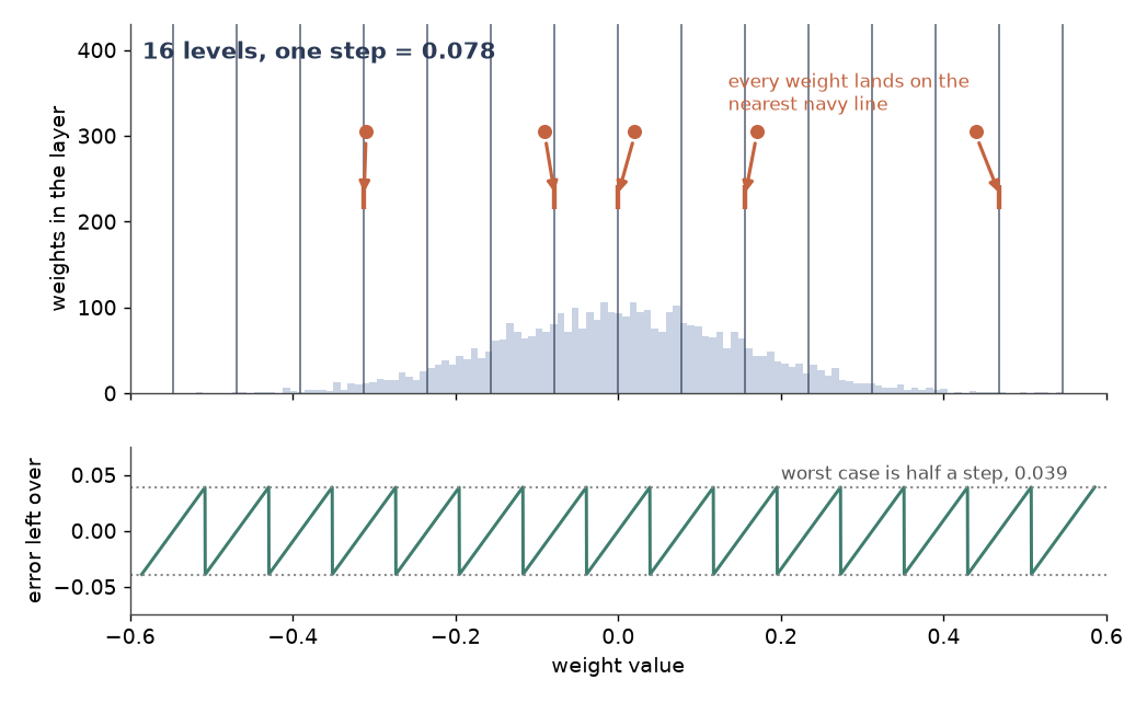Figure 1: One layer’s weights against the sixteen places a 4-bit number is allowed to be. Nothing clever is happening here. Every weight slides to the nearest navy line, and the sawtooth underneath is what it cost, which is at most half a step. Source: Author

Let’s do one block by hand, because the failure is easier to see in sixteen numbers than in seventy billion. Say the block is

0.08, -0.21, 0.35, -0.04, 0.12, 0.28, -0.31, 0.05, -0.17, 0.42, 0.09, -0.26, 0.19, -0.11, 0.33, -0.02

The largest magnitude is 0.42, so $s = 0.42/7 = 0.06$. Then 0.08 becomes notch 1 and comes back as 0.06, 0.35 becomes notch 6 and comes back as 0.36, -0.21 becomes notch -4 and comes back as -0.24. Nothing is off by more than 0.03, which is half a notch, and a weight matrix really does not notice 0.03.

Now swap one number. The fourteenth weight is no longer -0.11, it is 4.2, because one channel of this model has decided to shout.

The largest magnitude is now 4.2, so $s = 0.6$, and the ruler has been stretched to reach something only one weight needs. Eleven of the remaining fifteen weights now round to exactly zero, because they are all smaller than half a notch. The four survivors come back as $\pm 0.6$ whether they started at 0.31 or at 0.42. So one weight ate the whole block, and sixteen distinct numbers have become four, counting the big one.

That is the coat (an outlier channel).

The coat

There is always one thing in the pile that weighs as much as the rest of it put together. In a Transformer it is a handful of channels in the hidden state.

LLM.int8() (Dettmers et al., 2022) is the paper that measured them, and the shape of the finding is the interesting part. The outliers are not scattered about. In a 6.7B model there are roughly 150,000 outlier activations per sequence, and all of them sit in six feature dimensions out of four thousand. They turn up on nearly every token, at 20 to 100 times the magnitude of the median channel. They also arrive suddenly. Below about 6.7B parameters you can mostly ignore them, and above it you cannot.

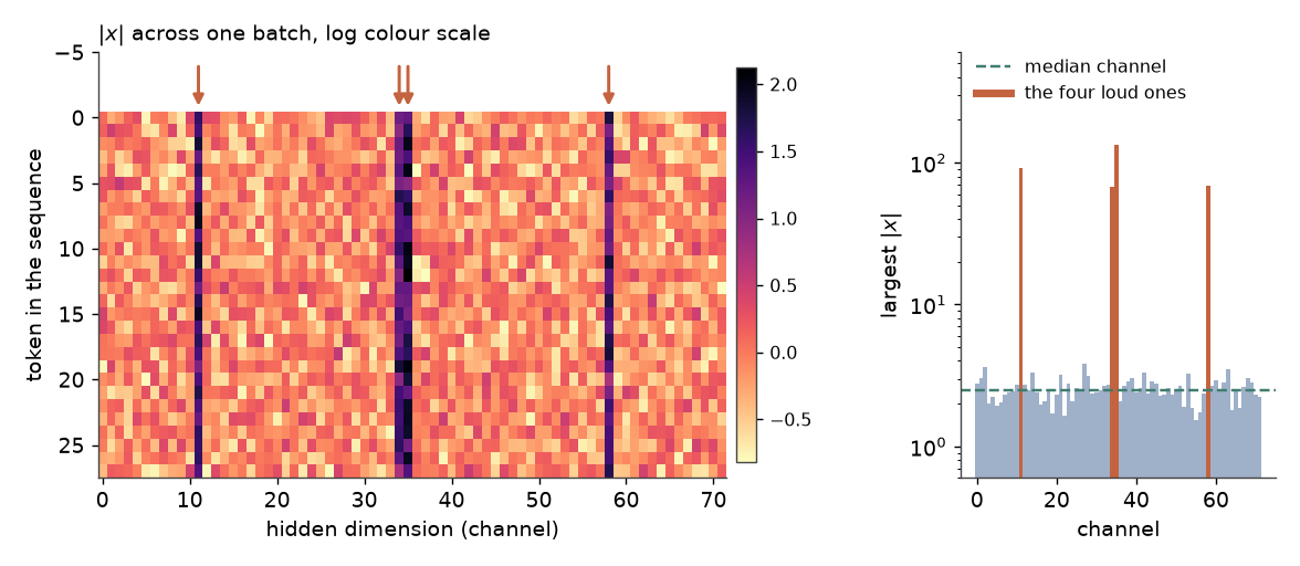Figure 2: What the hidden state actually looks like. The stripes are the same channels on every token, which is the only reason any of this is fixable. If they moved around, there would be no post here. Source: Author

Dettmers’ fix is the one you would use at the airport. You do not fold the coat into the bag. You wear it onto the plane, and it stops counting. LLM.int8() splits each matrix multiply in two: the outlier channels go through in 16-bit, everything else, which is more than 99.9% of the values, goes through in 8-bit, and the two halves are added back together. An OPT-175B checkpoint converts and runs with no measurable loss of quality, which in 2022 was the first time anybody could say that.

It also, quite often, ran slower than just using fp16.

That is the tension everything since has been working on. The airline does not care that you are wearing the coat, but a GPU does. A tensor core wants one big rectangular multiply of one dtype, and a ragged split into a fat INT8 part and a skinny FP16 part is two kernels, a scatter and a gather. So you save the memory and give back the time, which is a fine trade when you were out of memory and a silly one otherwise.

Three ways to not wear the coat

So how do you get the coat into the bag instead? There are three answers and every one of them is still in use, quite possibly in whatever you served a token from this morning.

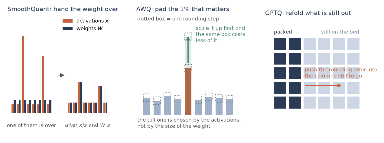Figure 3: The same problem, solved three ways. Move the weight to the bag that has room, pad the thing you care about, or refold everything you have not packed yet. Source: Author

Hand it to your travel partner. SmoothQuant (Xiao et al., MIT, 2022) notices that a matrix multiply does not care where the magnitude lives. Activations are spiky and weights are flat, so divide the activations by a per-channel number $t_j$ and multiply the matching weight rows by the same $t_j$. The product is identical. But the spike is now spread across two bags, and both are under the limit. The knob is the migration strength $\alpha$, which is how much of the difficulty you shove across, and 0.5 works for most models. That buys W8A8 on OPT-175B with no accuracy loss worth reporting, up to 1.56x faster and half the memory.

Pad the thing you care about. AWQ (Lin et al., MIT, 2023) starts from an observation that sounds too easy. Not all weights matter equally, and about 1% of the channels matter far more than the rest, because those are the channels the large activations run through.

Here is the ablation, and it is the best one in the quantization literature. Take OPT-6.7B at INT3 with groups of 128. Plain round-to-nearest gives a perplexity of 23.54 on WikiText-2, a standard slab of Wikipedia articles, against 10.86 for the original in FP16. That is a wreck. Keep 1% of the channels in FP16, chosen by the size of the activations flowing through them, and most of that gap closes. Now choose the same 1% by the size of the weights instead, which is the obvious thing to try, and you get about 22.4, so nothing at all. The size of a weight tells you almost nothing about whether it matters, and the size of what runs through it tells you almost everything.

AWQ then drops the mixed precision, because of the ragged-kernel problem above. It scales the salient channels up before rounding and folds the inverse into the previous layer, so one rounding step covers proportionally less of the number you cared about. Everything stays one dtype and the OPT-6.7B number lands at 11.39.

Refold as you go. GPTQ (Frantar et al., ISTA, 2022) quantizes a weight matrix one column at a time, and after each column it adjusts every column still to come, so they absorb the error the last one made. The adjustment is second-order, from an approximation to the layer’s own Hessian, which is a lot of machinery for “repack the rest of the bag after each thing you put in”. And it is quick: OPT-175B and BLOOM-176B both go through in about four GPU hours on one A100. At 4 bits the perplexity moves by 0.03, and at 3 bits from 8.34 to 8.68. That was the first method that let a 175B model run on a single 80 GB card, 3.25x faster than fp16.

How many labels are you carrying

All three of those methods still have a scale somewhere, and a scale is a number you have to store and fetch along with the weights. So the real knob is how many weights share one.

One scale for the whole tensor is the cheapest and the worst. One per output channel is the old default. One per group of 128 is what the GGUF file on your laptop does. And the current answer, microscaling, is one scale per block of 16 or 32, which is small enough that a single loud weight (an outlier) can only ruin its own block and its fifteen neighbours.

So why not go all the way and give every weight its own scale? Because an 8-bit scale attached to a 4-bit weight is a 12-bit format with extra steps, and you have spent a month of engineering to make the model bigger.

I ran the experiment for this post, on 65,536 normal weights with 0.2% of them made 30 to 60 times bigger, quantized to 4 bits:

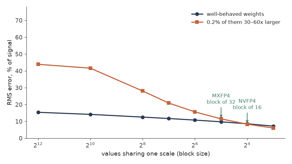Figure 4: What a block size buys you, for 4-bit symmetric quantization. With one scale per 4096 values, rare outliers cost 44% RMS error against 15% for well-behaved weights. By a block of 16 the two lines have met at about 8%, and the outliers have stopped mattering. Source: Author

Small blocks are not free either, because the scales are weights too. Let’s count. MXFP4 is a block of 32 values in E2M1 with one 8-bit power-of-two scale, so $4 + 8/32 = 4.25$ bits per weight. NVFP4 is a block of 16 with an 8-bit scale that is a real float rather than a power of two, so $4 + 8/16 = 4.5$ bits. Four and a half bits per weight, which is a lovely thing to say out loud to a hardware engineer and watch what happens.

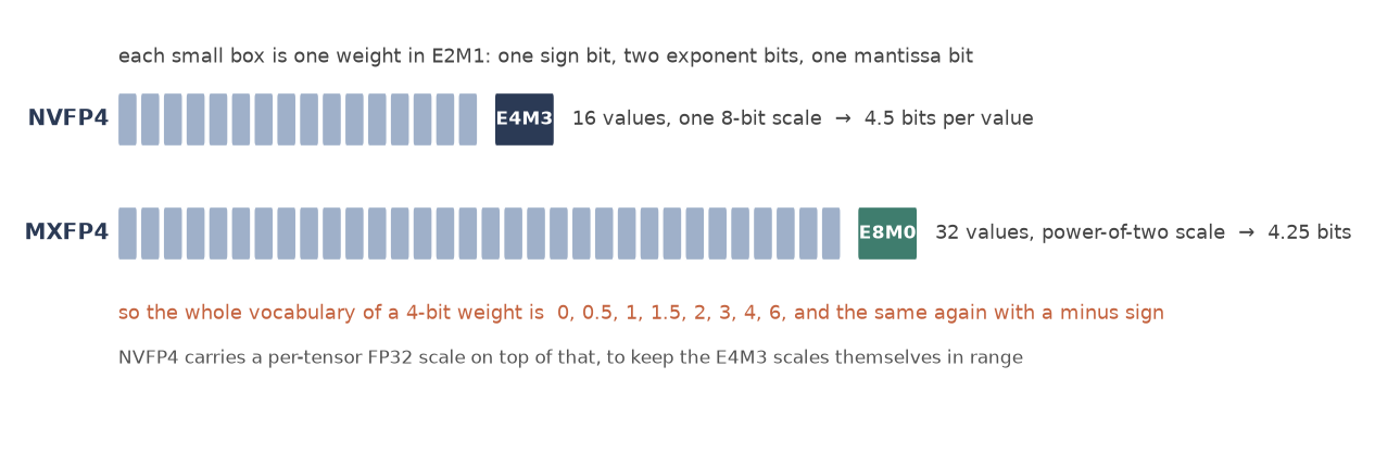Figure 5: The two 4-bit formats, laid out. Sixteen codes per weight, fifteen distinct values because zero is in there twice, and everything else in the format is about the scale sitting next to them. Source: Author

Format	Block	Scale	Effective bits	Verdict
INT4, per-tensor	whole tensor	one FP16	4.0	fine until a model gets big enough to shout
INT4, group 128	128	FP16 scale and zero	4.25	what your laptop runs, and it is good
MXFP4	32	E8M0, power of two	4.25	an open standard, and it rounds the scale too
NVFP4	16	E4M3, plus a per-tensor FP32	4.5	quarter of a bit dearer, and it wins

The power-of-two scale in MXFP4 is the interesting weakness. A block whose largest value is 1.1 gets a scale of 2, so the block is quantized as though its biggest member were nearly twice what it is, and half the grid goes unused. NVFP4 pays an extra quarter-bit for a scale that can say 1.125, and gets most of its accuracy advantage from that plus the shorter blocks.

Clothes that fold flat

Everything so far squashes a model that was trained in 16 bits. The other option is to train it in the format you mean to serve it in, so that it comes off the line already folded.

NVIDIA pretrained a 12B hybrid Mamba-Transformer on 10 trillion tokens in NVFP4 (2025) and got 62.58% on MMLU-Pro, a harder multiple-choice exam than the original MMLU, against 62.62% for the same recipe in FP8. Which is a rounding error, on a run that cost somebody several million dollars to be uncertain about.

The recipe needs three tricks, and they are all about the coat again:

1. Random Hadamard transforms on the inputs to the matrix multiply. A Hadamard rotation mixes every channel into every other one, so a single loud channel gets smeared across the block and stops setting the scale on its own. Same idea as QuaRot and SpinQuant, and it is now the first step of most quantization pipelines.
2. Two-dimensional scaling, so the weights are blocked the same way in the forward and the backward pass.
3. Stochastic rounding for the gradients. Round-to-nearest is biased when you apply it a trillion times to tiny updates, and a model whose updates are all smaller than half a notch stops learning. Round up or down at random instead, in proportion to where the value sits between two notches, and the bias goes away.

They also left the last few blocks of the model in higher precision, which is the part of every 4-bit paper that gets one sentence and deserves three.

Meanwhile the models arrive pre-squashed. gpt-oss-120b (OpenAI, August 2025) ships with its mixture-of-experts weights, which are over 90% of the parameter count, already in MXFP4, at about 4.25 bits each. That is why a 120B model fits on one 80 GB card. Quantization stopped being something you do to a release and became part of the release, and the same thing happened to fine-tuning back when QLoRA put a 4-bit frozen base model under a 16-bit adapter.

Where things are going

The other half of the bag. Weights are a fixed cost and the KV cache is the one that grows with your context. KIVI (2024) found the cache needs two different treatments: keys quantized per channel, because keys have channel outliers exactly like activations do, and values per token, because they do not. Everything since is a variation on that split.

Silicon deciding the format. FP4 tensor cores arrived with Blackwell in 2025 and exist nowhere else. So the formats the hardware vendor ships are the formats the field will use, and the argument about 16 versus 32 element blocks is being settled by what fits in a register file.

Below four. BitNet b1.58 (Microsoft, 2024) gives every weight one of three values, $-1$, $0$ or $+1$, which is 1.58 bits, and a matrix multiply with no multiplications in it. You cannot get there by squashing a finished model, though. You have to train it that way from the first step, which is a large bet to place before you know the answer.

What you find out at the other end

Every packing decision feels fine in the bedroom. Here is the part where you arrive.

Perplexity does not see the damage. This is the one I would put in front of anybody about to ship a quantized model. Quantized reasoning models think they need to think longer (2026) ran GPTQ and AWQ at 3 and 4 bits across five reasoning models. At 3-bit AWQ, accuracy on MATH-500, which is 500 competition maths problems, falls from 85.6% to 47.0%. And the chain of thought grows from 5.2K tokens to 23.4K. So it got worse and more expensive at the same time.

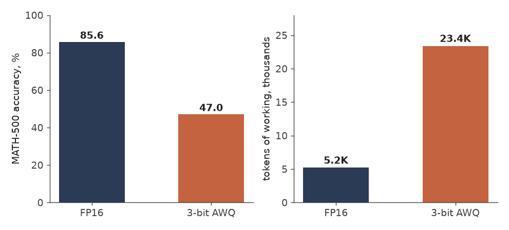Figure 6: The same model, quantized to 3 bits, as reported by the paper. Half the accuracy and four and a half times the tokens, from a change that barely moves a perplexity number. Source: Author

Why? Because in up to 52% of the failures, the model reached the right answer somewhere in its working and then talked itself out of it. The authors traced it to the positions where the next-token distribution is nearly flat, which is exactly where a rounding error gets to decide the outcome. At those positions the quantized model reaches for “wait”, “but” and “alternatively” more often than it should. So it can still do the maths, it has just stopped trusting itself, which is not a failure mode I expected a rounding error to have. A logit penalty on those specific tokens, with no retraining at all, cuts 12 to 23% off the length while keeping the accuracy.

More training makes a model harder to squash. Scaling Laws for Precision (Kumar et al., ICLR 2025) fitted 465 pretraining runs and found that the damage from post-training quantization grows with how many tokens the model saw. Past some point, more pretraining data actively hurts the quantized version of your model. Nobody likes this result, the runs behind it top out at 1.7B parameters, and it has been argued about ever since. But it predicts something real, which is that a recipe validated on last year’s checkpoint owes you nothing on this year’s.

The gate agent has the final say. A 4-bit model on hardware without FP4 units is a storage format. Your kernel unpacks each weight to 16 bits on the way to the tensor core, so you get the memory saving and the bandwidth saving, which is most of the win, and precisely none of the arithmetic saving. On an A100 that is still worth doing. It is also not what the vendor’s slide said.

And the calibration set is doing more work than anybody admits. GPTQ and AWQ both need a few hundred sample sequences to decide which channels matter, and those samples are usually a scrape of general web text. Calibrate on WikiText, deploy on Tamil legal contracts, and you have picked the important channels for somebody else’s job.

Conclusion

The bag has been the same size since 2022 and the pile on the bed keeps growing, so all of the progress here is in how you fold. Sixteen notches instead of sixty-five thousand, one scale per sixteen weights instead of one for the whole tensor, a rotation so no single channel gets to set the ruler, and a rounding rule that is wrong at random rather than wrong in the same direction every time.

What is different in 2026 is that the folding moved upstream. Models now arrive in four bits, trained that way on purpose, rather than being squashed by whoever has to serve them. So the question stopped being how small you can get a model and became which parts of it were ever worth sixteen bits. On the evidence so far that is the last few blocks and the odd loud channel, which is not many.

Everything else in this post is the same evening it always was. You will get the bag shut. The frame at the gate does not negotiate, the coat goes on over your arm, and you will discover somewhere over the Atlantic which of the eleven things you rounded to zero you actually needed.

And now you know. Fin.