
On the cover: the goods lift in the Fagus factory at Alfeld, installed in 1912 to carry shoe-last blanks between the floors. The cage makes the same trip whether it holds one blank or a full load, which is the whole trick of this post. Photo by Waltraud.gropius, CC BY-SA 4.0.

In the KV caching post we stopped the Transformer re-reading its own homework. Cache every key and value, squeeze the cache down to a latent with MLA (multi-head latent attention), and the quadratic bill for a long context turns into something a finance team will sign off on.
Then you serve the model, and it writes about twenty-four words a second.
The arithmetic is not what is slow. A 70B model needs roughly 140 billion multiply-adds to produce one token, and an H100 gets through that in about a seventh of a millisecond. Then it sits there for another forty-two milliseconds dragging the weights out of memory, so it can do the same thing again for the next word.
Welcome to the era of speculative decoding. This is the story of how you get three tokens for the price of one without touching a single weight, and how the thing that comes out is provably the same text the model would have written on its own.
I want you to picture a basement archive with a goods lift. The weights are the archive, 140 gigabytes of filing kept downstairs because there is nowhere else to put it. The archivist (the big model) has to walk the entire length of the stacks before he can answer anything at all, and the walk takes forty-two milliseconds. It takes forty-two milliseconds if you send down one question, and it takes forty-two milliseconds if you send down eight. The walk is what costs, and the questions weigh nothing. Since 2017 we have been sending that lift (one forward pass) down with a single sheet of paper on it.
What forty-two milliseconds buys
You might think the fix is a faster chip. Let’s do the sum first.
Take Llama-3-70B in bfloat16, a 16-bit number format. Seventy billion parameters at two bytes each is 140 GB of weights. To produce one token, every one of those bytes has to move from HBM (the high-bandwidth memory stacked next to the chip) onto the chip itself. An H100 SXM shifts 3.35 TB/s, so the floor is:
\[\frac{140\ \text{GB}}{3.35\ \text{TB/s}} \approx 41.8\ \text{ms per token} \approx 24\ \text{tokens/s}\]No kernel anybody writes will beat that, because it is not a software number. Now let’s price the arithmetic. One token is about $2 \times 70\text{B} = 140$ GFLOPs, and the H100’s bf16 units do 990 TFLOPs a second. So that comes to 0.14 ms. The ratio is roughly three hundred to one, and you have bought the most expensive arithmetic unit on the market to do arithmetic 0.34% of the time.
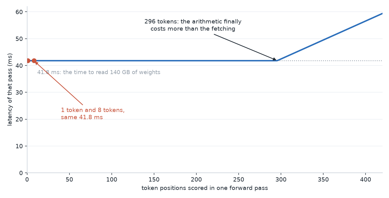 Figure 1: The roofline floor for one forward pass of a 70B model on an H100, against how many token positions you score in it. Scoring eight costs what scoring one costs. This is the floor and real kernels sit above it, so read the flat part as “nearly free” rather than “free”, which is still the best deal in the building. Source: Author
This is why batching exists at all: run sixty-four users through the same forward pass, and one walk answers sixty-four questions (which is how your API call comes to be quietly sharing a chip with sixty-three strangers). It is also most of why MoE pays, since a sparse model only fetches the experts it routes to. Both attack the same bill from the same side. But neither does anything for one person sitting alone waiting for their reply, because a batch of one is still one sheet of paper on the lift.
So the lift is going down anyway. What else can we put on it?
Guess, then check
Here is the whole idea, with no brand names in it yet.
Keep a second, much smaller model on the same machine, a 1B beside the 70B. Call it the pocket edition (the draft model): an abridged copy of the archive that sits on your desk, wrong a fair amount of the time and completely unembarrassed about it. Then, per round:
- The pocket edition writes the next $\gamma$ tokens onto a slip, one at a time. It has 2 GB of weights, so each of its steps takes about 0.6 ms.
- Send all $\gamma$ guesses down in one trip. The big model (the target) scores every position in a single forward pass. That is the same operation it does during training, and it costs exactly as much as scoring one position.
- Walk the slip from the top. Accept tokens while the big model agrees, stop at the first one it does not.
- At that first disagreement the big model writes the token itself, from the numbers it already computed.
Step 4 is the part that makes the accounting work. Even a slip where every single guess is rejected, still comes back with one correct token on it. That is precisely what an ordinary decoding step would have given you, so the worst round in the world costs you nothing you were not already spending.
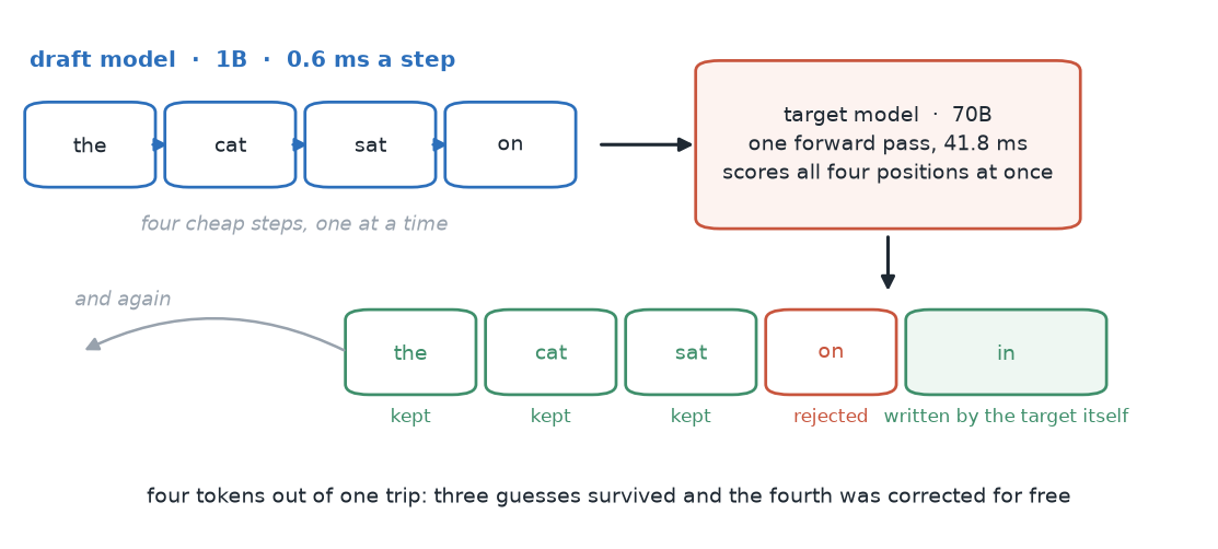 Figure 2: One round. The draft model runs four cheap steps, the target model runs one expensive one, and three tokens come back from a trip that used to carry one. Source: Author
In words, what you get per trip is:
\[\text{tokens per trip} = \frac{1 - (\text{chance a guess survives})^{\text{guesses} + 1}}{1 - (\text{chance a guess survives})}\]specifically,
\[\mathbb{E}[\text{tokens}] = \frac{1 - \alpha^{\gamma+1}}{1 - \alpha}\]where $\gamma$ is how many tokens the draft model wrote, and $\alpha$ is the acceptance rate, the probability that any one guess survives the check.
The correction that makes it exact
If you only ever want the greedy token, this is pretty easy: compare argmaxes, keep the matching prefix. That is blockwise parallel decoding (Stern, Shazeer and Uszkoreit, 2018). It bolted extra output heads onto a Transformer and did all of this five years before anybody cared, at NeurIPS, to approximately no applause.
Sampling is harder, and this is where the idea earns its keep. The draft model proposes token $x$ from its distribution $q$, and the big model has its own distribution $p$ over the same position. The two disagree by construction, because if they agreed you would not need the big one. Accepting whenever $p$ is merely non-zero, would quietly hand you the small model’s taste. So Leviathan, Kalman and Matias (Google, 2023) and, independently, Chen et al. (DeepMind, 2023) use a modified rejection sampling rule:
\[x \sim q(x), \qquad \text{accept with probability } \min\left(1, \frac{p(x)}{q(x)}\right)\]and when it is rejected, do not simply resample from $p$. Sample from what is left over:
\[x \sim \frac{\max(0,\ p(x) - q(x))}{\sum_{x'} \max(0,\ p(x') - q(x'))}\]where the numerator is the mass the big model wanted to put somewhere the small model did not, and the denominator just makes it sum to one. So why not skip the fuss and resample from $p$ whenever a guess is rejected? Because the rejected guesses are not a random sample. They are the ones $q$ over-proposed, so drawing fresh from $p$ on top of that would double-count everything the small model already got right. Subtracting first is what fixes it. The result is a theorem rather than a hope: the token you emit is distributed exactly as $p$. And the whole apparatus is the rejection sampling from a first-year statistics course, wearing a lanyard.
Let’s do one by hand, because the cancellation is the nicest thing in the paper. Say the vocabulary has four tokens, and the pocket edition (draft) has just proposed “the”:
| Token | Pocket edition (draft) $q$ | Archivist (target) $p$ | What happens |
|---|---|---|---|
| the | 0.60 | 0.30 | proposed; accepted with probability $0.30/0.60 = 0.5$ |
| a | 0.20 | 0.40 | under-proposed, so it collects 0.20 of residual mass |
| my | 0.15 | 0.20 | collects 0.05 |
| your | 0.05 | 0.10 | collects 0.05 |
The guess gets rejected with probability $1 - \sum_x \min(p,q) = 1 - 0.70 = 0.30$, and the residual distribution is $[0, 0.667, 0.167, 0.167]$. So the chance you finally emit “the” is $0.60 \times 0.5 = 0.30$, which is exactly $p(\text{the})$. The chance you emit “a” is $0.20$ from acceptance, plus $0.30 \times 0.667$ from the residual. That is $0.40$, which is $p(\text{a})$. Every row lands on $p$ exactly.
That $\sum_x \min(p,q)$ is worth a second look, because it is the acceptance rate. One minus it is the total variation distance between the two models, the biggest disagreement they can have about any set of tokens. The gap that cross entropy charges you as a loss during training, is the same gap charged here as a rejection probability at inference. Fail to teach the small model the big one’s taste, and you pay for it in wasted trips instead of wasted epochs.
How many guesses go on the slip
Now the only knob, which is the slip length $\gamma$. Longer slips mean more free tokens when the draft is good, and more binned paper when it is not. And the draft model’s own steps are cheap rather than free. Leviathan’s version, with $c$ as the ratio of one draft step to one target step:
\[\text{speedup} = \frac{1 - \alpha^{\gamma+1}}{(1 - \alpha)(c\gamma + 1)}\]Let’s put our two models in it. The 1B draft is 2 GB against 140 GB, so $c \approx 0.014$. Say $\alpha = 0.8$, which is roughly what a well-matched pair gets on ordinary prose. At $\gamma = 5$ the expected tokens per trip is $(1 - 0.8^6)/0.2 = 3.69$, and the round costs $41.8 \times (1 + 5 \times 0.014) = 44.7$ ms. That is 12.1 ms per token against 41.8, a 3.4x speedup, from a model you did not retrain, on hardware you already own.
Now let’s break it, because the failure teaches more than the win does. Keep the same 70B but draft with a 7B, which sounds sensible and gives $c = 0.1$. Then point it at a domain it was never trained for, say legal contracts, so that $\alpha$ falls to 0.3. Now the expected tokens per trip is 1.43, against a round that costs half as much again, and the formula returns a speedup of 0.95x. You have added a second model, a rejection sampler and a fortnight of engineering, and made your inference slower.
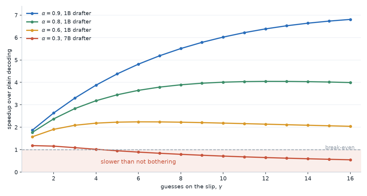 Figure 3: Speedup against slip length at four acceptance rates. The returns bend over fast: at $\alpha = 0.6$ you have had almost everything on offer by five guesses, and the mismatched pair from the paragraph above is a small win at two and a loss by five. Source: Author
This is not a hypothetical. Leviathan’s group measured acceptance rates from 0.53 to 0.82 across their T5 draft models, and reported an end-to-end 2x to 3x on T5-XXL. Chen’s group got 2x to 2.5x on Chinchilla 70B. Those are the honest numbers for a pair of models that were never designed for each other. Everything since has been an attempt to raise $\alpha$.
Where the guesses come from
So where does a draft model come from, if nobody has trained you one? That is the trouble with the separate-model version: somebody has to have built it, on your tokeniser, ideally on your data. Meta ships a 1B alongside the 70B, and life is good. Your fine-tuned radiology model does not come with a little sibling, and training one is a project.
Hence the hunt for drafts that fall out of the target model itself.
Medusa (Cai et al., 2024) is Stern’s 2018 idea with better manners: freeze the model, bolt on a few extra heads that each predict a token some distance ahead, and have them propose several candidates at every position rather than one. Those candidates form a tree. A masked attention pattern (tree attention) lets the target verify every branch of it in the one forward pass it was going to do anyway. Medusa-1, which trains only the new heads, reports over 2.2x. Medusa-2, which fine-tunes the model along with them, gets between 2.3x and 3.6x.
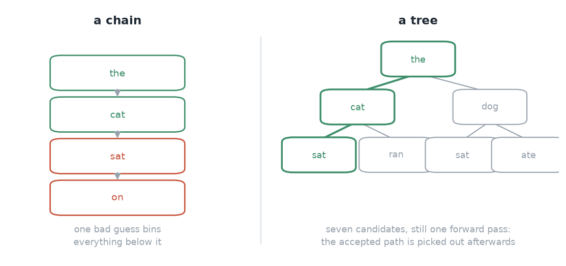 Figure 4: A chain commits to one guess per position, so one bad token bins everything after it. A tree hedges, and since verification is nearly free you may as well send several slips down together. Source: Author
EAGLE (Li et al., 2024) moves the drafting one level down. Instead of predicting tokens, it predicts the target model’s own second-to-top-layer features and reads a token off them. That is a better thing to guess, because features are what the model actually computes with, and they are smoother than the vocabulary. EAGLE-2 makes the draft tree adapt its shape to how confident the drafter is. EAGLE-3 abandons feature prediction, fuses features from several layers, and trains the drafter against its own multi-step outputs. It reports up to 6.5x on the HumanEval coding benchmark, with an average of 7.5 accepted tokens per trip. Seven and a half tokens is most of a clause, and the archivist is still doing one walk.
The drafter has its own lift
Every method above still has the draft model generating its guesses one at a time. Eight guesses is eight forward passes of the small model. Each is cheap on its own, but together they are the one piece of the round that grows when you make the slip longer, because the drafter has its own lift to ride.
DFlash (Z Lab, UCSD, 2026) attacks that. The drafter is a block diffusion model conditioned on hidden states pulled from the target. It denoises an entire block of 8 to 16 candidate tokens in one forward pass, instead of walking them out left to right (8 to 16, and nobody has yet explained to me what is wrong with 12). Integrated into vLLM’s TPU path and measured on a v5p with Llama-3.1-8B-Instruct, it reports 3.13x average tokens per second, and close to 6x on the MATH-500 maths set. The end-to-end serving speedup is 2.29x, where EAGLE-3 on the same rig managed 1.30x. On the MBPP Python set it takes 9.81 ms per token down to 3.48.
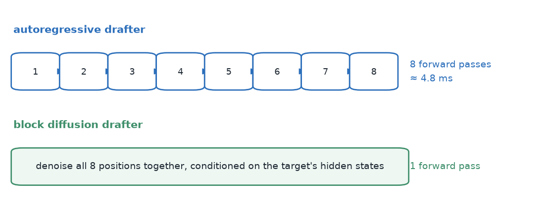 Figure 5: The drafter’s own bill. Eight guesses used to mean eight little forward passes; a block diffusion drafter fills the whole slip at once, which is the only piece of the round that was still strictly sequential. Source: Author
Which means the diffusion models that keep failing to displace autoregression as a way of writing text, have found honest work as the thing that guesses what autoregression is about to say. They were never great at being right on their own, but they are quick, and quick is all a drafter has to be.
| Method | Who writes the draft | Reported speedup | Verdict |
|---|---|---|---|
| Blockwise parallel (2018) | Extra heads on the model | ~2x, greedy only | Right five years early |
| Speculative decoding (2023) | A separate small model | 2x–3x | The one with the theorem |
| Medusa (2024) | Frozen model plus new heads | 2.2x–3.6x | No sibling model required |
| EAGLE-3 (2025) | Feature-level drafter, dynamic tree | up to 6.5x | Best acceptance anyone reports |
| DFlash (2026) | Block diffusion, whole block at once | 3.13x avg on TPU | Kills the drafter’s serial cost |
Every number in that third column was measured on different hardware against a different baseline, so read it as a rough ordering rather than a race.
Where things are going
MagicDec (CMU, 2024): MagicDec makes the point that at long context and large batch the KV cache becomes the thing you are hauling out of memory. So the bottleneck goes back to bandwidth, and speculation starts paying again exactly where the batch-size argument had written it off.
Scaling laws for drafters: EAGLE-3’s finding is that once you stop making the drafter predict features, throwing more training data at it keeps buying speedup instead of saturating. The draft model has become something you train properly rather than a spare part you had lying around.
Diffusion drafters: DFlash already has a queue of follow-ups behind it on arXiv, all with the same shape, which is to keep the exact verification and make the guessing parallel.
It is already underneath you: vLLM, SGLang and TensorRT-LLM all ship this, and the EAGLE 3.1 work landed in vLLM in May 2026. If you have used a hosted model this year, some of your tokens were guessed by something small before the big one signed them off.
The bill for the free ride
The free FLOPs are only free while nobody else wants them, and that is the con that actually matters. At batch size one the box is bandwidth-bound, and verifying eight tokens costs what verifying one costs. Push the batch to thirty-two and the linear layers become compute-bound. At that point the verification pass is doing thirty-two times $\gamma$ tokens of real arithmetic, and you are paying for every one of them. Serving teams measure speculative decoding going negative in that regime. That is why the 3x headline numbers in this post nearly all come from single-stream latency benchmarks, and why serving stacks now turn speculation off adaptively as load rises.
“Lossless” is also a claim about the distribution, and not about your output. Same distribution does not mean the same tokens come out. It does not mean bit-identical either, because a batched verification pass sums its floating point in a different order than a single-token pass does. Your regression tests will drift, and nothing will be broken.
An empirical anatomy of the thing on consumer hardware (2026) is the study to read before promising your manager anything. Across five draft-target configurations on a laptop, the best reached 1.61x at a slip length of six. Per-position acceptance fell from 69.7% for the first guess to 37.8% by the sixth. And three of the five configurations came out slower than plain decoding, for one of two reasons:
- The draft model failed to actually out-run the target.
- The quantised backend ran the “parallel” verification serially, which is a wonderful way to lose a week.
And the pocket edition occupies memory. Two gigabytes of drafter is two gigabytes you are not giving to the KV cache, which on a long-context workload is the resource you were short of in the first place.
Conclusion
The archivist was never the bottleneck. He is quick and he is right, and he happens to work at the bottom of a shaft that takes forty-two milliseconds to descend, whatever you put in it. Everything in this post is a way of putting more paper on the lift: a cheap abridged copy upstairs writing guesses (the draft model), a tree of them instead of a line (Medusa, EAGLE), a diffusion model filling the whole slip at once (DFlash), and one piece of rejection sampling at the bottom of the shaft that makes the archivist’s stamp count for exactly as much as if he had written every word himself.
The series question comes back around with a stranger answer than usual. We spent three posts asking whether attention was all we really needed. Here the honest reply is that attention had nothing to do with it. Speculative decoding does not change the attention pattern, the positions, the routing or a single learned parameter. It changes how many words you are allowed to ask for per trip to the basement, and it turns out that was worth a factor of three.
So the next time somebody tells you their model does 24 tokens a second, ask what it was doing for 41.6 of every 41.8 milliseconds.
And now you know. Fin.