Popular models for object detection - a brief study

On the cover: YOLO v5 applied on an Avengers Endgame poster; oh also, Rocket wouldn’t like being called a ‘dog’ huehue

Object detection is one of the classical problems in deep learning for computer vision only next to image classification. The goal of object detection is to locate the objects present in an image, in addition to classifying them. This includes predicting bounding boxes for localization and probability scores for classification of all the objects present in the image. If the outputs are segmentation masks instead of bounding boxes, then it’s called an instance segmentation task.

There is a lot of research done in this area and it can be overwhelming to remember all the important details. If only I had a dollar for everytime I forgot what YOLO or Faster R-CNN does and had to read the paper again :3 Hence, this blog post strives to quickly summarize the popular architectures that gave shape to this field. This article is not a tutorial, rather aummary to jog your memory of the following models: R-CNN, Fast R-CNN, Faster R-CNN, YOLO v1, v2, v3, RetinaNet, Mask R-CNN and FPN. There are more recent models such as EfficientDet and MonbileNet variants which I’ll try to cover in the future versions of this article. Relevant links are provided for reference and the images for model architectures are taken from the respective papers. Most of these architectures are tested on the PASCAL VOC dataset (2007, 2012) and recently on COCO dataset as well. Popular metrics to evaluate the object detection task is Average Precision (AP) and mean Average Precision (mAP)

R-CNN (2013): paper

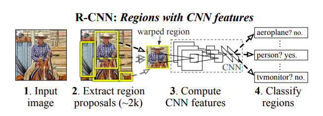R-CNN architecture This is one of the earliest deep learning architectures from Ross Girshick to address the object detection problem

1. Use Selective search algorithm to propose candidate regions (~2000 boxes)
2. Warp the candidate regions to a fixed size
3. Use a CNN model (eg. VGG-16) to extract features from these warped regions
4. Train C SVMs (one for each class, C classes) for object classification
5. In addition, bounding box regression is used to adjust the proposal regions (say a region proposal only covers half of a car)
6. During inference, use a greedy non-maximum supression to choose one box prediction from multiple predictions for a single object

Fast R-CNN (2015): paper

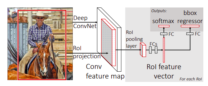Fast R-CNN architecture Training and inference on an R-CNN takes a long time as each of the 2000 warped regions undergo a forward pass through a CNN without sharing any computations. Thus the main author of R-CNN proposed this improved architecture.

1. Use an algorithm to propose candidate regions (~2000 boxes)
2. Produce a conv feature map of the input image using a CNN (eg. VGG-16)
3. Extract the projections of region proposals on the conv feature map using the reduction ratio (eg. say input is 256x256 and feature map is 32x32, then the reduction ratio is 1/8; say a proposal is 40x16, then the extracted projection is (40x16)/8 = 5x2 on the feature map at the corresponding location)
4. Use an RoI pooling layer on these extracted projections to produce a fixed size smaller feature map (7x7 in this paper)
5. Feed each of these fixed length feature maps/vectors into a sequence of FC (fully connected) layers
6. Feed the output of FC layers into two sibling layers: a softmax layer for object classification yeilding C probabilities and a class specific bbox regressor yielding 4C offsets for C classes

Faster R-CNN: paper

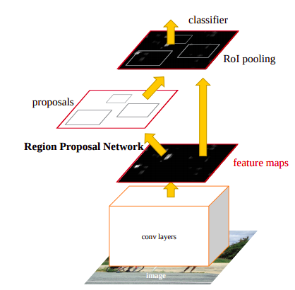Faster R-CNN architecture Same as Fast R-CNN but the region proposals are now done by a fully convolutional Region Proposal Network (RPN)

1. Extract a feature map of the input image (say conv5 of VGG) which is common to two parts of this network: RPN and a Fast R-CNN
2. The RPN uses a sliding window of fixed size (3x3 in this paper) to extract a 512-d output (conv5 of VGG has 512 channels as well) at each pixel of the feature map 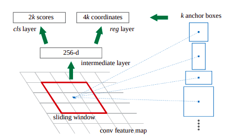RPN architecture
3. This is then connected to two sibling FC layers that predict k bounding boxes: 2k objectness scores and 4k coordinate offsets of k anchor boxes (a predetermined set of boxes with various dimensions and aspect ratios; k=9 in this paper)
4. For training RPN: the anchors as positive if IOU wrt to a ground truth>0.7 (if this fails, the anchor with the highest IOU is positive), negative if IOU<0.3 or ignore otherwise; a single ground truth can assign multiple positive anchors
5. Pass these proposals into a Fast R-CNN which has an RoI pooling layer and subsequently regress bboxes and predictions
6. In the paper, RPN and Fast R-CNN (for detection) are trained separately; RPN serves as an attention mechanism

YOLO: paper

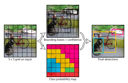Visualizing YOLO 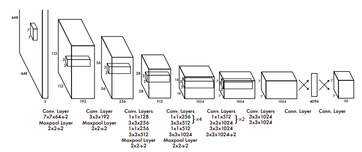Yolo architecture; YOLO reaches 45 fps (mAP 63.4 on 07 VOC) compared to Faster RCNN which reaches only 7 fps (mAP 73.2 on 07 VOC) A single unified end-to-end architecture from Joseph Redmon and Ali Farhadi, unlike R-CNN models where the region proposals and predictions are separate. YOLO models are constructed to provide real-time detections and thus compromise on accuracy. However, future versions address this problem. The latest version is YOLOv5 from Ultralytics, but they haven’t released a paper yet (as of writing this article) and there are arguments surrounding the name YOLOv5 since the actual authors are not involved in this version.

1. Use Darknet instead of VGG-16 as feature extractor; also, note the dense FC layers in the architecture that allows only fixed size input images
2. Divide the input image into an SxS grid (S=7 in the paper)
3. For each grid, predict B (B=2 in the paper) bounding boxes (each bounding box has 5 predictions: 2 center coordinates (Xc, Yc), 2 dimensions (H,W) and 1 objectness score) and C (C=20 in VOC) class probabilities. Hence the output would be SxSx(5*B + C) tensor, ie., 7x7x30 tensor
4. The predictions Xc, Yc are assumed to be offset wrt the grid cell location and H, W are also offset wrt to the size of the image

YOLO v2: paper

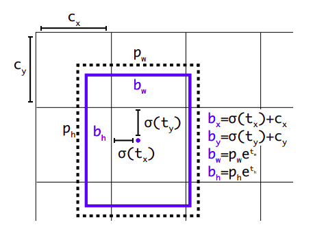YOLOv2 dimension priors and offsets using sigmoids and exponentials YOLO makes a significant number of localization errors. YOLOv2 tries to fix this. Similar to YOLO with following changes:

1. Higher resolution Darknet 19: base model pre-trained at image size of 448x448 instead of 224x224 (during object detection change size to 416 to get odd number of locations in the feature map (13x13) for a single cell center)
2. Add Batch Normalization to all the conv layers
3. Remove FC layers in YOLO and use anchors for prediction; cluster anchor box dimensions (using k-means; k=5 in this paper) on VOC and COCO instead of handpicked dimensions of 3 aspect ratios and 3 sizes
4. At each cell in feature map 13x13 (for a 416x416 input), predict k bounding boxes (for k anchors) and for each bounding box predict 5 values (2 center coordinates, 2 dimensions and 1 confidence)
5. Direct and stable bounding box location prediction using sigmoids and exponentials (in the image above)
6. Use a skip connection for fine-grained feature learning; to skip and concatenate a higher dimension layer of size 26x26x512, convert and stack it into 13x13x2048 for concatenation with the last layer
7. Multi-scale training of sizes (288, 320, 352, 384, 416, .., 544, .., 608) (multiples of 32 as that is the reduction size) for robustness to different image sizes (Note: YOLOv2 is independent of input image size, since you are predicting anchors at every cell of the feature map and no FC layers in the feature extraction step)

YOLO v3: paper

Incremental improvements over YOLOv2:

1. Use DarkNet53; Each bounding box predicts exactly one ground truth; assign the ground truth box to bounding box if the corresponding anchor box has the highest overlap and more than 0.5 IOU
2. Binary cross-entropy loss for each class (to predict overlapping classes eg., Woman, Person) instead of softmax and multi class cross entropy
3. Use FPN (Feature Pyramid Network) like feature pyramid predictions at 3 scales (the 9 clustered anchor box sizes are split evenly across these scales); the output tensor for the scale of size NxN is N×N×[3 ∗ (4 + 1 + 80)]; 80 classes
4. There’s also a Yolov3-tiny variant (has the highest fps) and a Yolov3-SPP variant (yields higher mAP score)

RetinaNet: paper

RetinaNet architecture

1. Use Feature Pyramid Network as the backbone to extract rich multi-scale feature pyramids
2. Then pass this into a classification subnet and a bbox regression subnet (both FCNs without sharing parameters) with anchors to predict boxes and classes
3. This is a dense prediction where you predict these bboxes for every pixel of the feature map as opposed to sparse predictions in Faster R-CNN
4. Use focal loss to account for object to background class imbalance in the data for single level detection

Mask R-CNN: paper

People have started to care more about segmentation masks than bounding boxes :)

1. Has the same architecture as that of Faster R-CNN
2. In addition to predicting bbox and class probabilities, it has an FCN (Fully Convolutional Network) attached at the end with deconvolution layers for predicting masks
3. Since there needs to be a one-to-one input image to feature map alignment, RoI Align) is used instead of RoI Pooling (which does harsh quantizations); RoIAlign is the main ingredient of Mask R-CNN

Feature Pyramid Network: paper

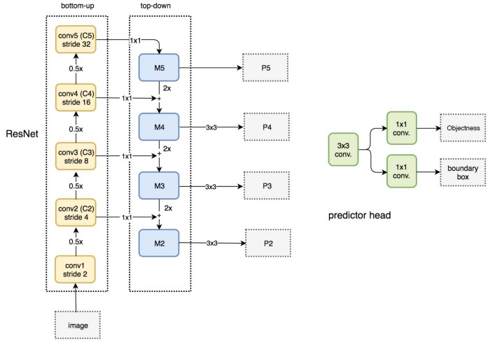FPN architecture VGG-16 is historically used for feature extraction. These days, FPN is adopted as the defacto feature extractor for obtaining fine-grained/multi-scale features.

1. Provides a multi-scale rich feature pyramid; nice explanation here
2. Contains a bottom-up pathway (normal ResNet feature extraction) and a top-down pathway (constructing pyramids). Top-down pathway is explained as follows for a 5 layer ResNet: (P satnds for pyramid)
   • P5: Use the last layer outputs: C5, channel size N-d, and convert them to 256-d channels using 1x1 convolutions
   • P4: Upsample P5 (x2) with the nearest neighbor upsampling to get the same spatial resolution of C4; convert C4 to 256-d by 1x1 convs; now merge these two: P4 = upsampled(P5) + 1x1convolved(C4)
   • P3, P2 same procedure used for P4
3. Do a 3x3 convolution in order to avoid aliasing effects after each merge
4. P1 is not constructed as it is too large for computations

Question: How do these models fare with different image sizes?

This is a typical question that arises while studying these models. This is answered here nicely. R-CNN and YOLO cannot handle various image sizes, since they have fully connected layers as part of the feature extraction network. Fast R-CNN (thus also Faster R-CNN; RPN is fully convolutional) allows different input image sizes beacuse of RoI pooling that outputs fixed size smaller feature maps for all the proposals. YOLO v2 onwards the models can process arbitrary inputs sincec they use anchor boxes at each cell. These days most architectures allow variable input image sizes as input because of these techniques in them:

FCN and SPP:

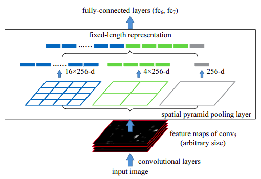SPP architecture; 256 is the filter number of the conv5 layer, and conv5 is the last convolutional layer

1. Both these techniques allow one to use varied size input images unlike traditional Imagenet models that consume only fixed size inputs
2. Fully Convolutional Networks (FCN): Use 1x1 convolutions instead of dense connections and finally use Global pooling at the end
3. Spatial Pyramid Pooling (SPP): This maintains spatial information in local spatial bins. This is similar to RoI pooling, in that they produce fixed size outputs. Effectively, define three bin sizes (1, 4, 16) for pooling the last feature map of arbitrary size (HxWx256 dimensions). For each of these bin sizes pool the feature map. Concatenate these fixed size pooled features then use dense connections at the end.