
On the cover: the wall of drawers at an ironmonger’s in Soignies, Belgium, with one of each part fixed to the front of its drawer. Point at the thing in your bag and you have found the drawer, no name needed. Photo by Jean-Pol GRANDMONT, CC BY 3.0.
.JPG)
Near every big market, there is a street of shops selling parts for things you already own. Washing machine drums, mixer couplings, the little rubber ring inside a tap. One of those shops has forty thousand items in it and no shop floor at all. Just a counter, and a wall of drawers going up to the ceiling.
Two kinds of people walk in. The first has a part number, GSK-441, read off the old part or out of a manual. The second has the old part itself in a plastic bag. It is the rubber ring that goes round the washing machine door, he says, and it has gone hard. The kitchen floor is wet.
Both of them want the same drawer. Only one of them can name it.
Welcome to the era of hybrid retrieval. This is the story of two completely different ways to find a thing, why each one fails exactly where the other works, and what it costs to run both and then referee them.
Every search box you have used this week is that counter. Something cheap runs over the whole shop and comes back with a shortlist, and then something expensive runs over the shortlist. The design is about pushing as much work as possible into the part that happens before you ask.
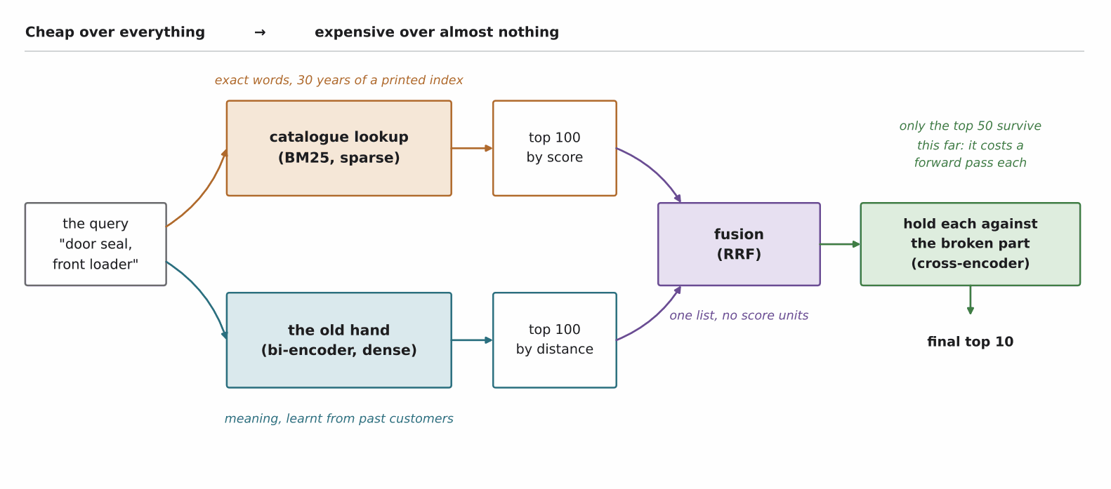 Figure 1: the four stages, and the budget behind them. Everything to the left of the fusion box has to be cheap enough to run on all forty thousand drawers. Source: Author
What the catalogue knows
Behind the counter there is a catalogue, and it is sorted by word rather than by drawer. Look up “seal” and you get a list of every entry that contains the word, with the drawer numbers printed next to it. Look up “door” and you get another list. The answer to “door seal” is what the two lists have in common. The lists are kept in order, so finding that is one walk down both at once. That is why this half stays fast however big the shop gets.
That is an inverted index, and it is the oldest idea in this post. For each word in the vocabulary, keep the list of documents containing it. The same tokenizer question applies here too, because somebody had to decide that “door” and “doors” are the same entry and “GSK-441” is one word rather than two.
Having the list is not the same as having an order, though. If four hundred entries say “seal”, somebody has to decide which one goes on top. The ranking function that nearly everybody still uses to decide is BM25, from a 1994 paper called Okapi at TREC-3 by Stephen Robertson and colleagues at City University London. BM is for best matching. The 25 is said to be the twenty-fifth formula they tried, though I have never seen a citation for that. Okapi was their retrieval system. It is also a forest animal that looks like somebody assembled a giraffe out of spare parts, which for this post is almost too convenient.
BM25 is three ideas sitting in one fraction, and all three are things the man behind the counter already does.
- A rare word is worth more than a common one. “GSK-441” appears in one entry. “Machine” appears in nine thousand. If you say both, only one of them has told him anything.
- Saying a word again stops helping. An entry that says “seal” four times, is not four times more about seals. It is probably just a longer entry.
- A long entry has to work harder. A forty-word description has more chances to contain your word by accident than an eight-word one.
In words, an entry scores well when it contains your rare words, without having needed many words to do it. Specifically,
\[\text{score}(q, d) = \sum_{i=1}^{n} \text{IDF}(q_i) \cdot \frac{f(q_i, d)\,(k_1+1)}{f(q_i, d) + k_1\left(1 - b + b\,\dfrac{\vert d \vert}{\text{avgdl}}\right)}\]where $q_i$ is the $i$-th word of your query, $f(q_i, d)$ is how many times entry $d$ contains it, $\vert d \vert$ is the entry’s length in words, and avgdl is the average entry length across the whole catalogue. The rarity term is its own small formula,
\[\text{IDF}(q_i) = \ln\left(\frac{N - n(q_i) + 0.5}{n(q_i) + 0.5} + 1\right)\]with $N$ the number of entries in the catalogue and $n(q_i)$ the number of them containing the word. There are two knobs. $k_1$ sets how fast repetition stops paying, and $b$ sets how hard long entries are punished. Almost everybody ships $k_1 = 1.2$ and $b = 0.75$, including Elasticsearch (nobody I have asked can tell me why those two numbers rather than some others).
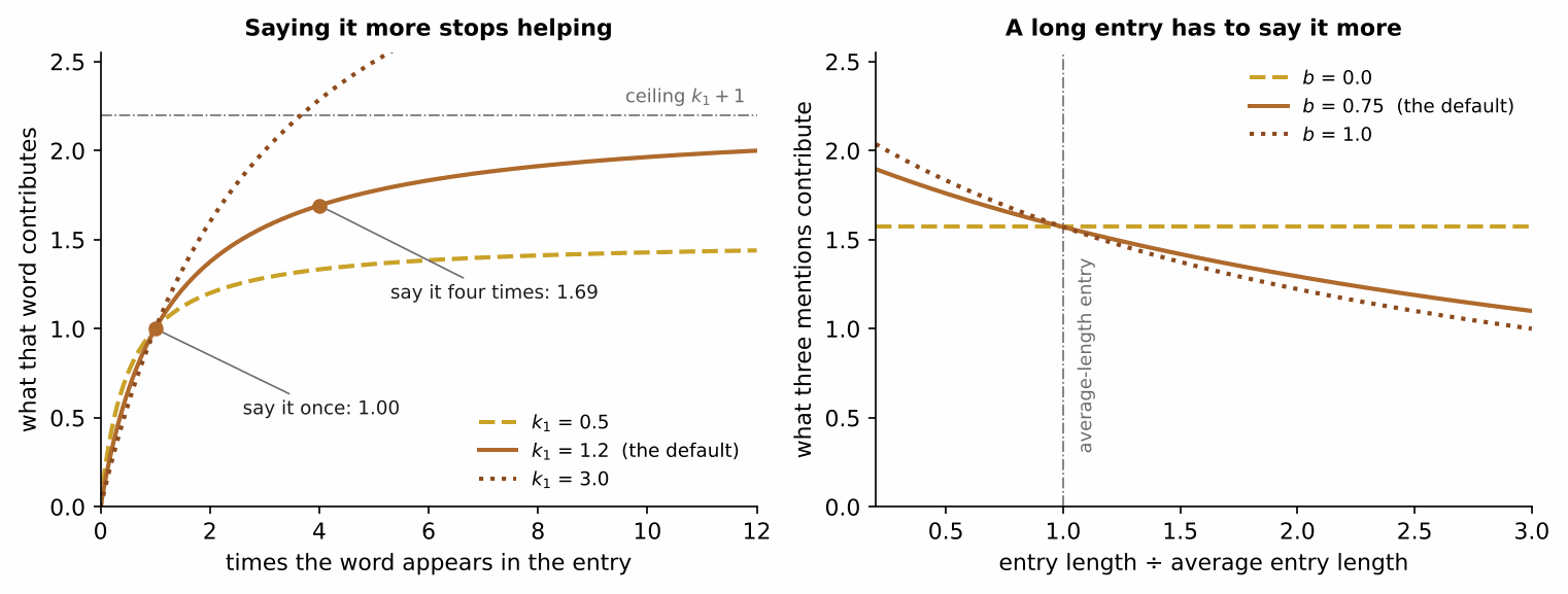 Figure 2: the two knobs. The left curve flattens because of $k_1$, the right one slopes because of $b$. Set $b$ to zero and length stops mattering at all, which is occasionally what you want and usually a bug. Source: Author
Let’s do one by hand. Say the catalogue has $N = 1000$ entries, the average entry is 12 words, and you ask for “door seal”. The word “seal” is in 120 entries and “door” is in 300, so their rarity scores are 2.12 and 1.20. The rarer word is worth about 1.8 times the common one before anything else happens.
Now two candidate entries. Entry A is eight words, “Door seal, front loading washing machine, rubber gasket”, and says each of your words once. Entry B is a forty-word catch-all that says “seal” four times and never says “door”. Running the fraction gives A a score of 3.84 and B a score of 2.55, so A wins. These scores have no ceiling and no units. They mean something against each other, inside this one query, and nothing at all outside it.
And look at what B got for its four mentions. Set the rarity number aside and run just the fraction: one mention in a short entry comes out at 1.16, and four mentions in a long entry at 1.21. Four times the word, four percent more credit, which is the saturation and the length penalty eating the repetition between them.
A real catalogue holds millions of entries rather than a thousand, and the only thing that changes is how large the rarity numbers get. This is a word count from 1994 with two constants in it. It has no idea what a seal is, it cannot be trained, and it is still the baseline that embarrasses people in 2026.
The customer who does not know the word
Here is what the catalogue cannot do.
A woman comes in and says the black ring round the washing machine door has gone hard and the water comes out at the bottom. Not one word of that is in the catalogue entry, which calls the thing a door gasket, front-load, EPDM. She said ring, it says gasket. She said black, it says EPDM. The lists come back empty, or worse, full of entries about doors.
This is the vocabulary mismatch problem. Two people describing the same object, pick different words for it. An index built on words has no way to know they meant the same drawer. So how do you look a thing up by what it does, when the customer cannot say what it is called? You can paper over it with a synonym list, and people did, for about thirty years. Somebody maintains that list by hand, and it is wrong in a new way every time a manufacturer renames something.
The old hand
The man who has worked there thirty years does not look anything up. He hears “black ring, door, water on the floor” and walks to a drawer. He has heard ten thousand customers describe things badly, and he has learnt a map from the way people talk to the place things live.
That is dense retrieval, and the map is an embedding. A neural network (the encoder) reads a piece of text and emits a single vector of a few hundred numbers. Dense means every one of those numbers is doing work, as against the catalogue’s sparse version: a slot for every word in the vocabulary, almost all of them zero. Train it so that a question and the passage answering it land close together, and you have a lookup that works on meaning instead of spelling. The version everybody cites is Dense Passage Retrieval (Karpukhin et al., 2020), which used two BERT encoders, one for questions and one for passages. Two separate towers like that are a bi-encoder.
The training trick is cheap and worth knowing. You take a batch of question-passage pairs that belong together. Then you treat every other passage in the same batch as a wrong answer for your question. A batch of $B$ pairs hands you $B(B-1)$ negative examples for free, which is why these models are trained with the biggest batch the hardware allows. The loss is the same softmax over similarities that the cross entropy post spent two thousand words on.
It buys you an index you can build years in advance, because the passage side never sees the question. It costs you the ability to compare against all forty thousand drawers, because that many dot products on every keystroke gets expensive fast. That second problem is the whole subject of the HNSW post. You build a small-world graph over the vectors and walk it greedily. So you touch a few hundred of them instead of all forty thousand. That is an approximate nearest-neighbour search, approximate because the greedy walk can miss the true closest vector, and now and then it does.
Send the old hand to a different trade
DPR is very good at the thing it was trained on. On Natural Questions, a set of real Google queries with Wikipedia answers, it finds the right passage in its top 20 about 78.4% of the time against BM25’s 59.1%, a gain of 19.3 points. On those queries, the word count is simply beaten.
Then BEIR (Thakur et al., 2021) took eighteen retrieval datasets from different domains, and ran the same trained models against all of them without retraining. That is the zero-shot setting: no new examples, no fine-tuning, just the model walking into a trade it has never seen. Everything is scored with nDCG@10, a number between 0 and 1 for how much of the right material turned up in the top ten, counting the higher positions for more. The results are in Figure 3 and they are not subtle.
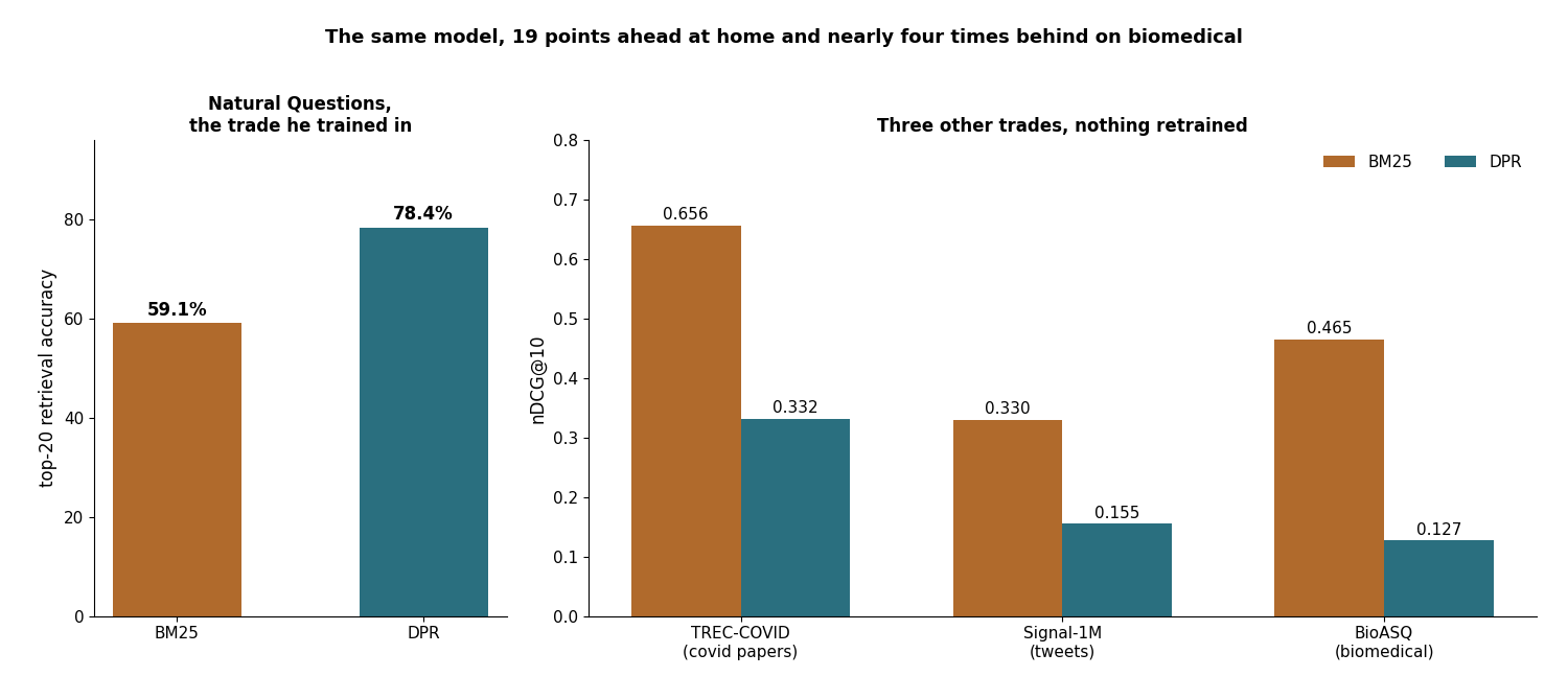 Figure 3: the same model in two situations. On biomedical questions it scores 0.127 against BM25’s 0.465, which is the sort of number you get from a system that has formed an opinion about words it has never seen. Source: Author
On BioASQ, a biomedical question set, BM25 scores 0.465 and DPR scores 0.127. On TREC-COVID it is 0.656 against 0.332. On Signal-1M, which is tweets, it is 0.330 against 0.155. Nineteen points ahead on the questions it trained for, nearly four times behind on biomedical, with no change to the model at all. Those are two different metrics, so the halves are not strictly comparable.
The reason is the one you would guess from the shop. The old hand learnt his map from the customers who actually came in. Put him behind a counter in a trade he has never served, where the words are drug names and gene symbols he has never once heard at this counter. He will still walk confidently to a drawer. He just walks to the wrong one. The catalogue has no feel for anything, which is exactly why it does not care that the trade changed.
Ask both, and then argue about the answer
So ask both, and merge the two lists. Why not just add the two scores together and sort? BM25 hands back scores like 14.2 and 9.8. They are unbounded sums, and they depend on how rare your words happen to be in this particular catalogue. The encoder hands back cosine similarities like 0.81 and 0.77. Those live between $-1$ and $1$, and in practice they bunch near the top, because the encoder was trained to pull anything vaguely related together. Adding 14.2 to 0.81 is adding rupees to rainfall. You can normalise each list first, by min-max or by z-score, and that works. But now the score of your third result depends on what else happened to be in the list that day.
The usual answer is to throw the scores away entirely. Reciprocal rank fusion looks only at the position of each document in each list. In words, a document’s fused score is the sum, over the lists it appears in, of one divided by a constant plus its rank. Specifically,
\[\text{RRF}(d) = \sum_{r \in R} \frac{1}{k + r(d)}\]where $R$ is the set of ranked lists, $r(d)$ is the position of document $d$ in one of them, and $k$ flattens the difference between the top few places. It comes from a two-page paper by Cormack, Clarke and Büttcher at SIGIR 2009, which beat the fancier merging schemes of the day, Condorcet voting among them, with one line of arithmetic.
The value of $k$ is 60. The authors fixed it during a pilot study, found it was near optimal, and never changed it. Every hybrid search stack you have ever queried runs on a constant somebody picked once, in 2009, before any of these embeddings existed.
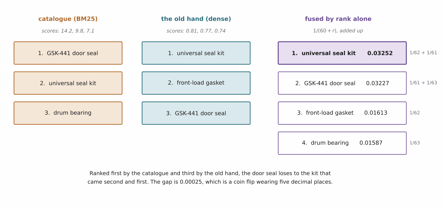 Figure 4: the whole algorithm, on four results. The right-hand column is the entire implementation. Source: Author
Now check Figure 4. The catalogue puts GSK-441 first and the universal kit second. The old hand puts the kit first and GSK-441 third. The kit scores $1/62 + 1/61 = 0.03252$ and GSK-441 scores $1/61 + 1/63 = 0.03227$, so the kit wins by 0.00025. Two lists disagreed, and the referee broke the tie by a margin that is a coin flip wearing five decimal places.
Does it work? Elastic ran it on BEIR by fusing BM25 with their learned sparse encoder, and reported an 18% lift in average nDCG@10 over BM25 alone and 1.4% over the sparse encoder alone. More useful is the other number they report: the fused result was at least as good as BM25 on every dataset they tried. That is what you are actually buying. Your search stops falling over on the day somebody types a part number into it.
Hold it against the broken part
Everything so far has been the shortlist. The man still has to walk to the counter with four candidates and hold each one against the thing in your bag.
That comparison is a cross-encoder. Instead of encoding the query and the entry separately, you glue them into one string and push them through a single model. So every word of the query can attend to every word of the entry, which beats one dot product between two summaries. And it is unusable for search, because nothing can be precomputed. The entry is only ever read next to this one query, so a corpus of forty thousand needs forty thousand forward passes.
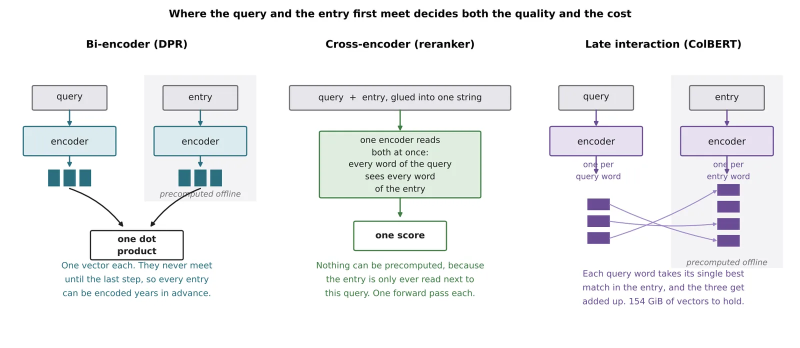 Figure 5: the same three boxes rearranged. The grey panels are what you can compute before the query arrives, and they are the entire reason the left-hand design is the one that touches your whole corpus. Source: Author
So you run it on fifty candidates rather than forty thousand, which is the retrieve-then-rerank pattern in Figure 1. On BEIR, BM25 followed by a cross-encoder reranker was the best configuration in the original paper, about 11% above BM25 on the average. Blog benchmarks for 100 candidates land around 45 ms for a small six-layer reranker and 130 ms for a large one. That is fine for a search box, and a problem for an agent that retrieves a dozen times before it answers.
There is a middle design. ColBERT keeps one vector per word of every entry instead of one per entry. At query time each query word takes its single best match, and the scores are added up. Most of the work is precomputed, and the query still sees the entry word by word. The cost arrives as storage: vanilla ColBERT needs about 154 GiB to index MS MARCO, a corpus of roughly 8.8 million web passages. That is tens of times the size of the text it indexes. ColBERTv2’s compression takes that to 16 GiB at one bit per dimension. The other middle design is SPLADE, which learns to write extra words into the catalogue entry. So the inverted index handles synonyms itself, and you keep the exact-match behaviour.
| Method | Matches on | Cost per query | Where it wins |
|---|---|---|---|
| BM25 | exact words, weighted by rarity | microseconds | part numbers, rare terms, any domain it has never seen |
| Bi-encoder | one vector of meaning each | one approximate nearest-neighbour search | paraphrase, the customer with no vocabulary |
| RRF of the two | positions in two lists | both of the above, run in sequence | never losing badly, which is the actual product requirement |
| Cross-encoder | every word against every word | a forward pass per candidate | the last fifty, after something cheap has chosen them |
| ColBERT | every word, best match per query word | storage, 154 GiB before compression | when you want the word-level comparison at index time |
Where this actually shows up
- Every retrieval-augmented generation (RAG) stack, which is now the main consumer of all of this. The ranked list goes into a model’s context window rather than onto a results page.
- Elasticsearch and OpenSearch ship RRF as a built-in query type. Vespa, Weaviate and pgvector all expose some flavour of hybrid.
- Code search, almost entirely the part-number case (nobody greps for the general vibe of a function), and enterprise and legal search, where the corpus looks nothing like the open web the embedding models trained on.
Where things are going
Embedding models have got much better at the zero-shot problem since DPR, mostly by training on far more and far more varied pairs. The gap in Figure 3 is narrower in 2026 than it was in 2021, though nobody has closed it on exact-match queries.
Learned sparse retrieval is the quieter trend and I think the more interesting one. If the index can expand “ring” into “gasket” at write time, you get the synonym behaviour inside the data structure that was already fast and auditable.
And rerankers are quietly becoming the whole game. Hand a language model the query and ten candidates and ask it to order them, and you get the cross-encoder’s every-word-against-every-word comparison from a model somebody else already paid to train. It is far slower than the 130 ms reranker. But if the model was going to read those passages anyway, you were buying that pass regardless.
The drawer marked miscellaneous
Every shop has one, and here is what is in mine.
The benchmark numbers here are softer than they look. Reproductions of BEIR disagree with each other. Pyserini gets 0.595 for BM25 on TREC-COVID with title and body indexed as one field. Index them as two and it gets the paper’s 0.656. On BioASQ the order flips, 0.522 against 0.465. And different papers average over different subsets of the eighteen datasets. So a method “2.5% above BM25 on average” may be above or below it depending on which of the eighteen you counted. I would not read a two-point difference between two retrievers as meaning anything.
Hybrid is also not free and not automatically better. One published comparison had an untuned hybrid scoring below its own dense-only baseline, 0.390 against 0.410 on mean reciprocal rank, which grades a list by how far down the first right answer sits. It only beat the baseline, at 0.486, once a weighted combination of the two scores was tuned. That is weighted fusion rather than RRF, which has no weight to tune. And that is rather the point, because the moment you want to favour one retriever, you are back to normalising scores. It is also a vendor-adjacent benchmark over 100 questions, so treat it as a direction rather than a measurement. Either way you run two queries instead of one. Elastic notes they go in sequence, which costs latency. And you keep two indexes in sync over the same documents.
RRF throws information away on purpose, and nobody talks about what that costs. A document BM25 scored 40 and one it scored 4.1, are identical to the referee if they both came third. When one retriever is confident and the other is guessing, RRF cannot tell, because confidence is exactly the thing it deleted.
The last one bothers me most. Almost nobody retrieves for a human reader any more. nDCG@10 is built on a model of a person reading down a list and losing interest, so it discounts position 9 heavily. But the consumer is now a language model that reads all ten, and a wrong-but-plausible passage at position 7 can do more damage to the final answer than an empty result would. We are tuning a ranking metric for a reader who no longer exists.
Conclusion
The two customers want the same drawer, and neither can be served by the other one’s method. A part number is pure rarity and no meaning, which is the easiest thing an inverted index will ever see. A description of a black ring that has gone hard is pure meaning and no vocabulary, which is the easiest thing an embedding will ever see. Thirty years of search was spent picking a side.
What shipped instead was both, a 2009 constant to referee them, and an expensive model that only ever looks at the last fifty. The fusion step earns its place on the day somebody types GSK-441 into a semantic search box, because something in the building still has to know what a number is.
My bet is that the two halves stop being two systems. Learned sparse retrieval is already an embedding model writing into an inverted index. We run two indexes only because nobody has built one data structure that is good at rarity and meaning at once. The day that exists, the referee goes away and the constant 60 retires after a long career nobody noticed.
Until then, bring the broken part. The man can read a number off it, and if there is no number, he can still see what it is for.
And now you know. Fin.