On the cover: An AI-generated image showcasing the capabilities of Flux models
In Part 1 of this series, we explored the basics of Flux models, their mathematical foundations, and how they compare to traditional diffusion models. Now, let’s dive deeper into the architecture, training process, and practical applications of these powerful new models. Congratulations on surviving the mathematical marathon of Part 1 btw! ;)
The Flux Architecture: Transformers Meet Flow
Now that we understand the theoretical foundations, let’s look at how Flux models implement these ideas in practice. Flux models use a novel architecture called Multimodal Diffusion Transformers MM-DiT in the same paper, that takes into account the multi-modal nature of the text-to-image task. Unlike previous transformer-based diffusion models, MM-DiT allows for bidirectional flow of information between image and text tokens, improving text comprehension and typography. It’s like upgrading from one-way walkie-talkies to actual phones - suddenly both sides can talk at once!
The architecture consists of:
- Multimodal transformer blocks: These process both text and image tokens, allowing for cross-modal attention (imagine Tinder, but for matching text descriptions with visual features)
- Parallel diffusion transformer blocks: These improve hardware efficiency and model performance (because why do things sequentially when you can do them all at once and crash your GPU in style?)
- Rotary positional embeddings: These help the model understand spatial relationships in the image (essentially giving the model a built-in compass so it doesn’t put dog heads on human bodies… usually)
Let’s break down the MM-DiT architecture a bit more:
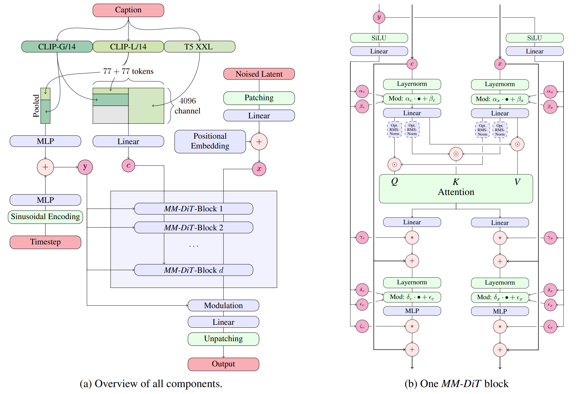 Figure 1: Full diagram of the MM-DiT architecture used in Flux models. If it looks complicated, that’s because it is. The researchers didn’t make it complex just to confuse you, but I’m not ruling it out either.
In traditional transformer-based diffusion models, text and image information flow in a unidirectional manner. The text conditions the image generation, but there’s limited feedback from the image back to the text representation. MM-DiT changes this by allowing bidirectional information flow, which helps the model better understand and implement complex text prompts.
The parallel attention layers are particularly interesting. Instead of processing attention sequentially, Flux models compute multiple attention operations in parallel, which significantly improves computational efficiency. This is crucial when scaling to 12 billion parameters. It’s the computational equivalent of multitasking - something I attempt while cooking dinner, answering emails, and burning said dinner.
Flow Matching at Scale
What makes Flux truly special is how it scales flow matching to massive model sizes. The researchers performed extensive scaling studies, showing that the performance of the model improves predictably with size, following clear scaling laws. Who could have guessed that bigger models perform better? Well, everyone, but now we have math to prove it!
The mathematical relationship between model size and performance can be approximated as:
\[\text{Performance} \approx a \cdot \log(N) + b\]where $N$ is the number of parameters, and $a$ and $b$ are constants.
This predictable scaling allowed the researchers to confidently build a 12 billion parameter model, knowing it would outperform smaller models.
Training
Training a Flux model involves several sophisticated steps, or as I like to call it, “how to burn through your cloud computing budget in record time”:
-
Data preparation: Curating a diverse dataset of image-text pairs. The quality and diversity of this dataset are crucial for the model’s performance.
-
Caption improvement: Using AI to generate better captions for images (similar to DALL-E 3’s approach). This technique, sometimes called “re-captioning,” involves using a separate model to generate more detailed and accurate captions for training images.
- Flow matching training: Learning to predict the velocity field between noise and data. For each training pair $(x_0, x_1)$, where $x_0$ is from the data distribution and $x_1 \sim \mathcal{N}(0, \mathbf{I})$, we:
- Compute the interpolation: $x_t = (1-t)x_0 + tx_1$
- Calculate target velocity: $v_t = x_1 - x_0$
- Train with loss: \(\mathcal{L}_{FM}(\theta) = \mathbb{E}_{t,x_0,x_1}\left[\|v_\theta(x_t, t) - (x_1 - x_0)\|^2\right]\)
- Rectification: Applying path straightening techniques by minimizing the path length: \(\min_{p(x_0, x_1)} \mathbb{E}_{(x_0, x_1)}\left[\int_0^1 \|v_t(x_t)\|^2 dt\right]\) where $v_t(x_t)$ is the predicted velocity field.
One interesting aspect of Flux training is the use of a technique called “Reflow.” After initial training, the model can be further refined by iteratively applying the flow matching process. Each iteration makes the paths between noise and data straighter, leading to more efficient sampling.
Sampling
The sampling process in Flux is remarkably simple, which is a pleasant surprise given how complex everything else has been:
- Start with random noise $z_1 \sim \mathcal{N}(0, I)$
- For each step $t$ from 1 to 0 (decreasing):
- Predict the velocity $\hat{u}(z_t, t)$ using the neural network
- Update: $z_{t-\Delta t} = z_t + \hat{u}(z_t, t) \cdot (-\Delta t)$
- Return the final image $z_0$
What’s impressive is that Flux.1 Schnell can generate high-quality images with as few as 1-4 steps, compared to the 20+ steps typically required by diffusion models.
A Deeper Comparison with Diffusion Models
You might be wondering: why does flow matching seem to work better than traditional diffusion? The answer lies in the mathematics of the two approaches. In diffusion models, we’re learning to predict the noise that was added to the image, which is an indirect way of learning the data distribution. In flow matching, we’re directly learning the vector field that transforms noise into data. This direct approach has several advantages:
- Simpler objective function: The flow matching loss is a straightforward L2 loss
- More efficient sampling: Straighter paths mean fewer steps are needed
- Better conditioning: The model can be more easily conditioned on text or other modalities
To further understand the differences, let’s compare the sampling processes of diffusion models and Flux models:
| Aspect | Diffusion Models | Flux Models |
|---|---|---|
| Sampling equation | \(x_{t-1} = \frac{1}{\sqrt{\alpha_t}} \left(x_t - \frac{1-\alpha_t}{\sqrt{1-\bar{\alpha}_t}} \epsilon_\theta(x_t, t)\right) + \sigma_t z\) | \(z_{t-\Delta t} = z_t + \hat{u}(z_t, t) \cdot (-\Delta t)\) |
| Complexity | More complex, involves multiple terms | Simpler, direct update |
| Stochasticity | Can be stochastic or deterministic | Typically deterministic |
| Path nature | Curved paths between noise and data | Straighter paths |
| Step count | 20-50 steps typically needed | 1-20 steps depending on variant |
The simplicity of the Flux sampling equation is striking. It’s essentially just following the predicted velocity field backward in time, which is both conceptually simpler and computationally more efficient.
Classifier-Free Guidance
Both models support classifier-free guidance (CFG) for better prompt adherence, but implement it differently:
-
Diffusion Models: Guide the score function \(\nabla_{x_t}\log p_t(x_t|y) = \nabla_{x_t}\log p_t(x_t) + w(\nabla_{x_t}\log p_t(x_t|y) - \nabla_{x_t}\log p_t(x_t))\)
-
Flux Models: Guide the velocity field directly \(v_\text{guided}(x_t, t) = v_\text{uncond}(x_t, t) + w(v_\text{cond}(x_t, t) - v_\text{uncond}(x_t, t))\)
The key advantage of Flux’s approach is that it maintains straight paths even with strong guidance, while diffusion models’ paths can become more curved with higher guidance scales. This helps explain why Flux can maintain efficiency even with strong conditioning. It’s like the difference between a GPS that recalculates your entire route when you make one wrong turn (diffusion) versus one that just gets you back on track with minimal detours (Flux).
Now that we understand the basics, let’s pit these two generative heavyweights against each other in a no-holds-barred comparison. Think of it as a mathematical cage match where only one approach can claim the generative crown (though in reality, they’re more like cousins than enemies).
| Aspect | Diffusion Models | Flux Models | Winner |
|---|---|---|---|
| Mathematical Foundation | Gradually adding and removing noise; predicting the noise that was added (score function) | Direct transformation between distributions; predicting the velocity field | Flux (for simplicity) |
| Process Nature | Stochastic process with curved paths from noise to data | Deterministic process with straighter paths | Flux (for efficiency) |
| Sampling Steps | 20-50 steps typically needed | 1-20 steps depending on variant | Flux (by a mile) |
| Image Quality | Good to excellent, improving with each generation | Excellent, with superior prompt adherence | Flux (slightly) |
| Hardware Requirements | Can run on consumer GPUs for older models | Needs high-end GPUs due to parameter count | Diffusion (for accessibility) |
If diffusion models are the reliable family sedan that gets you where you need to go, Flux models are the sleek sports car that turns heads while doing it faster. The trade-off? That sports car needs premium fuel (read: expensive GPUs). Diffusion models have been the workhorses of generative AI for good reason - they’re accessible, well-understood, and produce great results. But Flux models are showing us what happens when you take the mathematical scenic route and optimize for a straighter path between noise and data.
If there’s one area where Flux truly shines, it’s speed. While diffusion models typically need 20-50 sampling steps (with SDXL Turbo being the exception that proves the rule), Flux models - especially the aptly named Schnell variant - can generate high-quality images in as few as 1-4 steps. That’s not just an incremental improvement; it’s a paradigm shift that could make real-time generation a practical reality.
The biggest obstacle to Flux world domination? Hardware requirements. While you can run Stable Diffusion 1.5 on a modest gaming GPU with 8GB of VRAM, Flux models are resource-hungry beasts that typically demand A100 or H100 GPUs for optimal performance. It’s like comparing the computing requirements of a calculator to those of a space shuttle. This hardware barrier means that for many hobbyists and smaller studios, diffusion models will remain the practical choice for the foreseeable future. Flux is that rich friend who keeps telling you how much better their Tesla is than your Honda, while you silently calculate how many months of rent their car payment would cover.
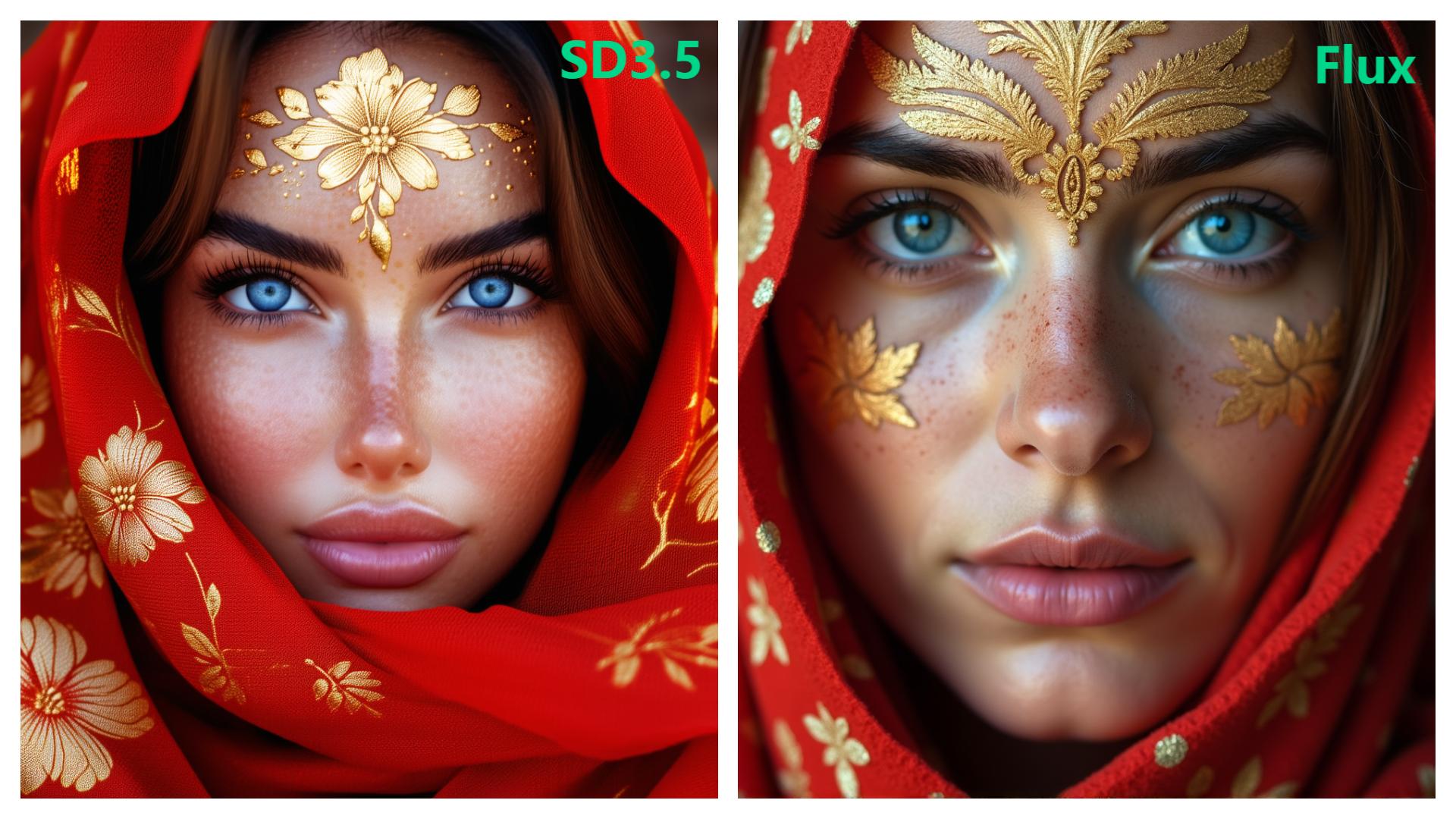 Figure 2: Comparison of images generated by Stable Diffusion 3.5 (left) and Flux.1 (right) For close-up faces, Flux delivers better detail, quality, and realism. Though to be fair, both are better artists than I’ll ever be.
Conclusion
Flux models represent a significant step forward in generative AI, combining the best aspects of transformers and flow matching to create a powerful new approach to image generation. By learning to directly model the transformation from noise to data, these models achieve better quality, faster generation, and improved prompt adherence.
As with any rapidly evolving field, it’s hard to predict exactly where this technology will lead. But one thing is certain: the flow of progress in generative AI shows no signs of slowing down. Whether Flux models will become the new standard or simply another stepping stone in the evolution of generative AI remains to be seen. But for now, they’re definitely worth keeping an eye on!
References
- Improving Image Generation with Better Captions - DALL-E 3 paper on caption improvement techniques
- Fine-tuning FLUX.1 with your own images - Guide to fine-tuning Flux models