
On the cover: A police sketch in progress, drawn from a description rather than a photograph
A witness sits down across the table. She was in the room. You want to know who else was.
You do not hand her a canvas and ask her to reproduce the scene. You ask her to describe the person. Tall, grey coat, walked with a limp. A sketch artist turns that into something you can circulate.
Her description throws away almost everything she saw: the wallpaper, the carpet, the light through the blinds, the pattern on the coffee cup. All of it gone and none of it missed, because none of it was ever going to help you find anybody.
Now, a computer vision model has the same choice to make, and for about a decade it made the other one.
Here’s the setup. We have oceans of unlabeled pixels and almost no labels. Self-supervised learning is the trick of inventing your own question so you don’t need a human to answer it, and the question the field settled on was fill-in-the-blank. Hide part of the input, predict the missing part, and whatever internal machinery the model builds to do that is the thing you actually wanted.
It is a great trick, it gave us BERT, and the trouble only starts when you ask what the model should fill the blank in with.
Welcome to Joint-Embedding Predictive Architectures, or JEPA. This is the story of how vision models stopped trying to paint the room and started trying to describe it.
We have been asking for a painting
Masked Autoencoders are the clean version of fill-in-the-blank for images. Mask 75% of the patches, reconstruct the missing pixels, and the loss is:
\[\mathcal{L}_{\text{MAE}} = \frac{1}{|\mathcal{M}|}\sum_{i \in \mathcal{M}} \|\hat{x}_i - x_i\|^2\]where $\mathcal{M}$ is the set of masked patches, $x_i$ the true pixels, and $\hat{x}_i$ the reconstruction. It works. It also asks the model to paint the wallpaper.
Think about where the gradient goes. Some of what’s behind that mask is genuinely predictable: if you can see three quarters of a dog, the fourth quarter is a dog. But most of the bits are noise. The exact grain of the tarmac, the speckle in the shadows, which way each leaf happened to be pointing at that instant. Those pixels are unpredictable in principle, and the loss punishes the model for missing them anyway.
So the model spends its capacity on the least informative part of the image, not because anyone designed it that way, but because pixels are where the entropy lives, and squared error goes looking for entropy (it is, at heart, a metal detector on a beach).
Video makes this worse rather than better, which is unfortunate, because video is the biggest pile of unlabeled data we have. A photo has no future to get wrong, but a clip does, and most of what happens in the next frame is unknowable at the pixel level even if you understand the scene perfectly.
So ask for the description instead, and see what breaks.
The anatomy of a JEPA
Yann LeCun sketched the blueprint in a 2022 position paper, A Path Towards Autonomous Machine Intelligence. Three parts, and everything since is a variation.
- A context encoder $f_\theta$, the witness who saw part of the scene.
- A target encoder $\bar{f}_\theta$, a second witness who saw a different part.
- A predictor $g_\phi$, the sketch artist, who takes the first witness’s description plus a note saying which part of the room you’re asking about, and guesses what the second witness would say.
The loss compares two descriptions and never touches an image:
\[\mathcal{L}_{\text{JEPA}} = \big\| g_\phi(f_\theta(x),\, z) - \bar{f}_\theta(y) \big\|^2\]where $x$ is the visible context, $y$ the hidden target, and $z$ the positional information telling the predictor what it’s being asked about.
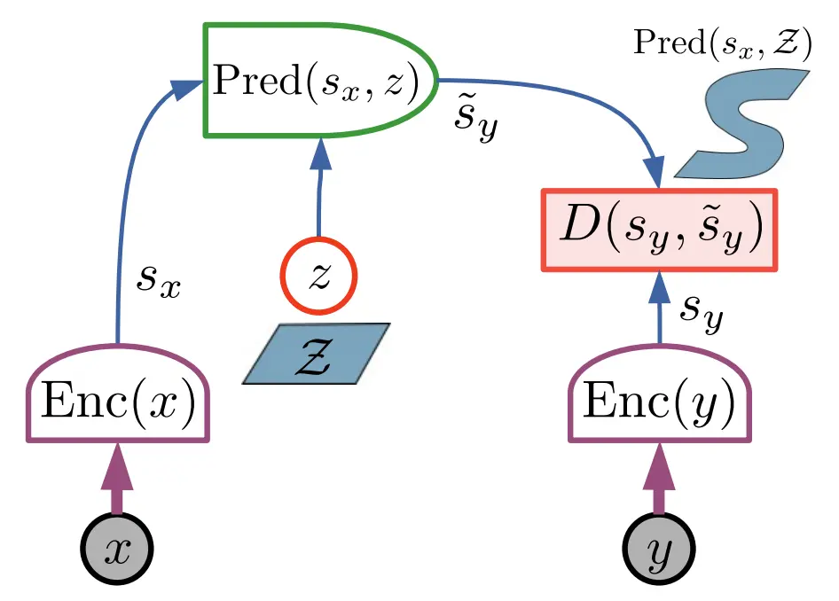 Figure 1: The JEPA blueprint. Two encoders turn $x$ and $y$ into descriptions $s_x$ and $s_y$, the predictor guesses $\tilde{s}_y$ from $s_x$ plus a latent $z$, and the energy $D(s_y, \tilde{s}_y)$ scores one description against the other. Nothing decodes back to pixels. Source: A Path Towards Autonomous Machine Intelligence
Notice what disappeared: there is no decoder anywhere, so the wallpaper doesn’t show up in the loss because the wallpaper doesn’t show up at all. Now notice what that costs, because it is the whole rest of this post.
The witnesses can collude
You are grading two witnesses on whether their descriptions agree. What is the laziest way to make two descriptions agree?
Decide in advance to say “a person, probably” about everything.
Formally: let the encoder learn the constant function $f_\theta(x) = c$ for every input $x$. The predictor learns the identity. Then
\[\mathcal{L}_{\text{JEPA}} = \|c - c\|^2 = 0\]That is zero loss at the global minimum with nothing learned, which is representation collapse, and it is the reason joint-embedding methods were considered cursed for years. Reconstruction never had this problem, because you cannot fake a photograph, whereas you can absolutely fake a description (ask anyone who has written a self-appraisal).
The fixes came in two families, and the difference between them matters more than anyone admitted at the time.
The first family separates the witnesses and hopes. BYOL puts a predictor head on one branch, makes the other branch an exponential moving average copy, and cuts the gradient to it:
\[\bar{\theta} \leftarrow \tau \bar{\theta} + (1-\tau)\theta\]with the decay $\tau$ usually somewhere around 0.996 to 0.999 (the gap between those two numbers has cost somebody a month, and I am glad it was not me). The target updates slowly, so the two can never quite settle on a shared story. SimSiam throws out the EMA and keeps the stop-gradient. DINO runs teacher-student distillation with centering pulling the output toward uniform and sharpening pulling it toward peaked, the two balanced by a schedule that somebody tuned.
Here is the part I find genuinely uncomfortable. None of this forbids collapse. The constant solution is still a perfectly valid global minimum of BYOL’s loss. It just doesn’t happen in practice, and the papers explaining why came out years after the methods, written by people who had been shipping them the whole time. We built foundation models on top of that.
The second family constrains the statistics instead. Barlow Twins pushes the cross-correlation matrix between two views toward the identity. VICReg says it out loud with three terms, an invariance term, a variance hinge forcing every dimension above a floor, and a covariance penalty to decorrelate:
\[\mathcal{L}_{\text{VICReg}} = \lambda\, s(Z, Z') + \mu\, [v(Z) + v(Z')] + \nu\, [c(Z) + c(Z')]\]These actually rule out the constant solution with no teacher required, and they deserve more credit than they got. Hold that thought, because it becomes the entire story in part 2.
NOTE: JEPA inherited family one wholesale. I-JEPA, V-JEPA and V-JEPA 2 all ship an EMA target encoder and a stop-gradient, and they keep the predictor deliberately narrow so it can’t do the job by itself.
I-JEPA: the first witness
I-JEPA (Assran et al., CVPR 2023) is the recipe made concrete for images.
Step 1: the interrogation
Sample one context block and four target blocks from the image, with the masks made disjoint so the context can’t peek at its own answer. The context encoder sees only visible patches. The target encoder sees the whole image, and the targets are slices of its output at the four masked locations.
The masking is not a detail, it’s the entire contribution, and the ablation is the good part. Target blocks have to be large and semantic, and the context has to be spatially spread out. Make the targets small and the model learns to answer “beige”, because colour and texture win. Make them big enough to hold an object part and the only way to answer is to have understood the picture.
The question has to be hard enough that guessing doesn’t pay. Any schoolteacher could have told them that.
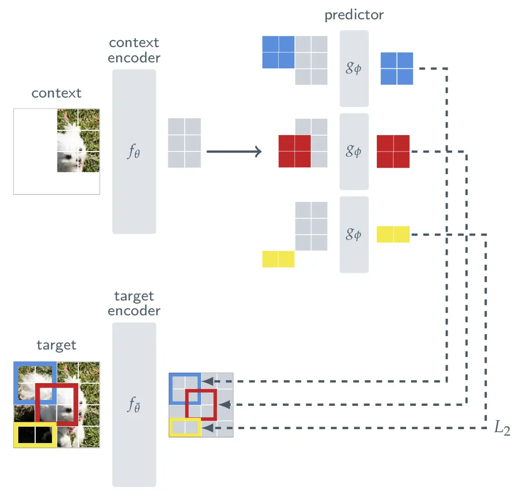 Figure 2: I-JEPA. One context block predicts the representations of several target blocks, with the predictor conditioned on positional tokens shown in colour. Source: I-JEPA
Step 2: the sketch artist
The predictor is a narrow ViT. Feed it the context embeddings plus a set of mask tokens carrying the position of the block you want, and it produces a guess at that block’s representation. Same predictor, different positional token, different answer.
Step 3: the verdict
Averaged L2 over all blocks and all patches inside them:
\[\mathcal{L} = \frac{1}{M}\sum_{n=1}^{M} \sum_{i \in B_n} \|\hat{y}_i - y_i\|_2^2\]where $M = 4$ is the number of target blocks, $B_n$ the patch indices in block $n$, $\hat{y}_i$ the predictor’s output and $y_i$ the target encoder’s. Gradients reach the context encoder and predictor only. The target encoder moves by EMA.
On ImageNet linear probing with a ViT-L/16, I-JEPA gets 77.5% against MAE’s 76.0%. The margin is small and I wouldn’t lean on it. What I would lean on is how it got there: without random crops or colour jitter, with no augmentation pipeline of any kind, which is the machinery every contrastive method of that era depended on. And a ViT-Huge/14 trained on 16 A100s in under 72 hours, which for a Meta vision paper is a suspiciously modest number.
V-JEPA: moving pictures
V-JEPA (Bardes et al., TMLR 2024) takes the recipe to video. The masks become tubes, a 2D mask extended through every frame of the clip, so the model can’t cheat by copying the same patch from next door in time. Training data was VideoMix2M, two million videos stitched together from Kinetics-710, Something-Something v2 and HowTo100M.
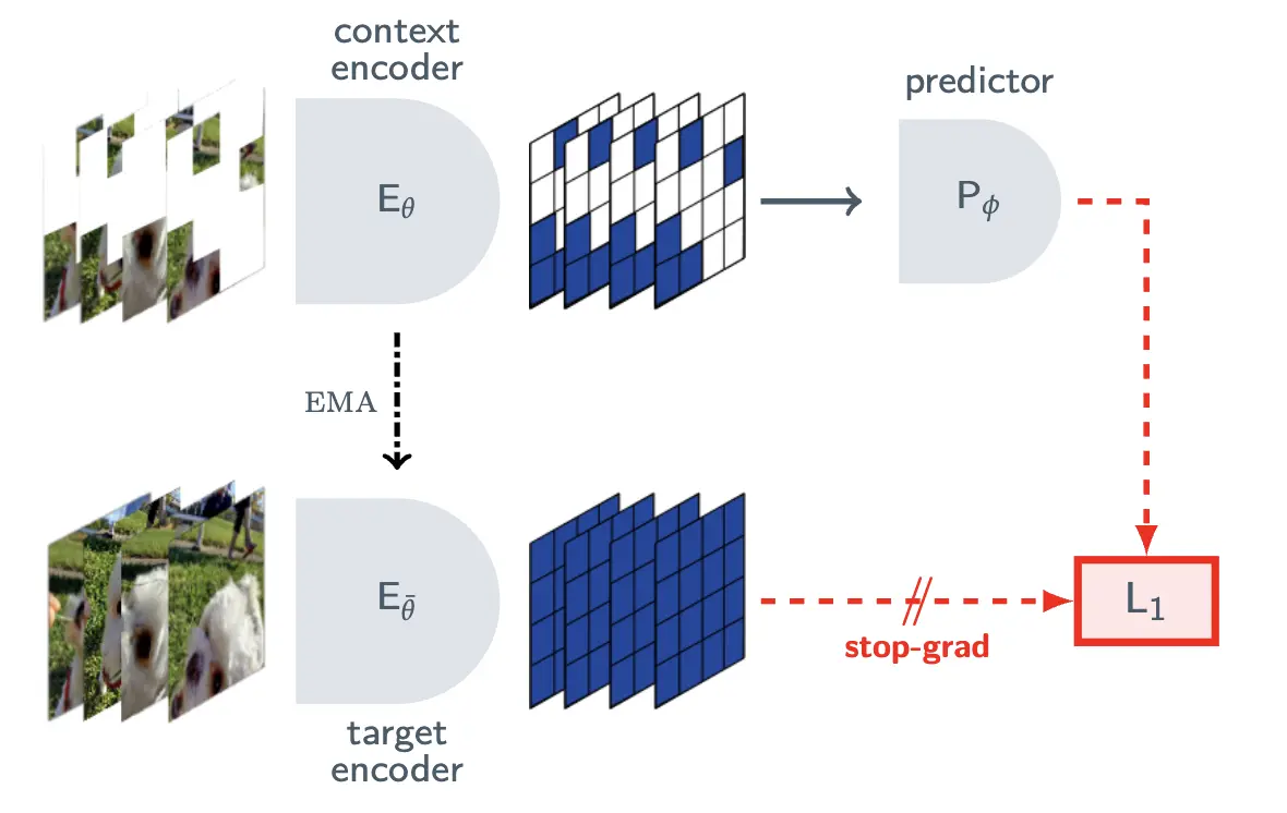 Figure 3: V-JEPA. The context encoder sees a tube-masked clip, the target encoder is an EMA copy fed the unmasked clip, and the stop-grad on the target branch is the thing standing between this and the constant solution. Source: V-JEPA
The number that matters is the frozen-backbone evaluation. No fine-tuning, just a probe on features that never move:
| Model | Kinetics-400 | Something-Something v2 | ImageNet-1K |
|---|---|---|---|
| V-JEPA ViT-H/16 | 81.9 | 72.2 | 77.9 |
| V-JEPA ViT-L/16 | 82.1 | 71.2 | — |
Something-Something v2 is the interesting column. Its classes are things like “uncovering something” and “pushing something so it falls off the table”, so recognizing objects gets you nowhere. You have to have understood the motion. With frozen features on SSv2, V-JEPA beats VideoMAEv2 by over 14 points.
The label-efficiency curve is the real tell though. The fewer labels you hand the downstream probe, the wider the gap gets against pixel reconstruction. That is exactly what you’d expect if one model has a description and the other has a photocopy.
V-JEPA 2: what happens with a million hours
V-JEPA 2 (Assran et al., 2025) stops being modest about compute. ViT-g encoder, over a billion parameters, trained on VideoMix22M: more than a million hours of internet video plus a million images (about 114 years of footage, so some of it is definitely cats). Two changes to the recipe, mask denoising with an L1 loss in place of straight mask prediction, and 3D rotary position embeddings.
- Something-Something v2: 77.3% top-1, against InternVideo2-1B at 69.7 and PEcoreG at 55.4
- ImageNet-1K: 84.6%, so specializing on motion cost nothing on appearance
- Epic-Kitchens-100 action anticipation: 39.7 recall@5, up 44% relative on PlausiVL’s 27.6
- Aligned with an LLM at 8B: 84.0 on PerceptionTest, 76.9 on TempCompass
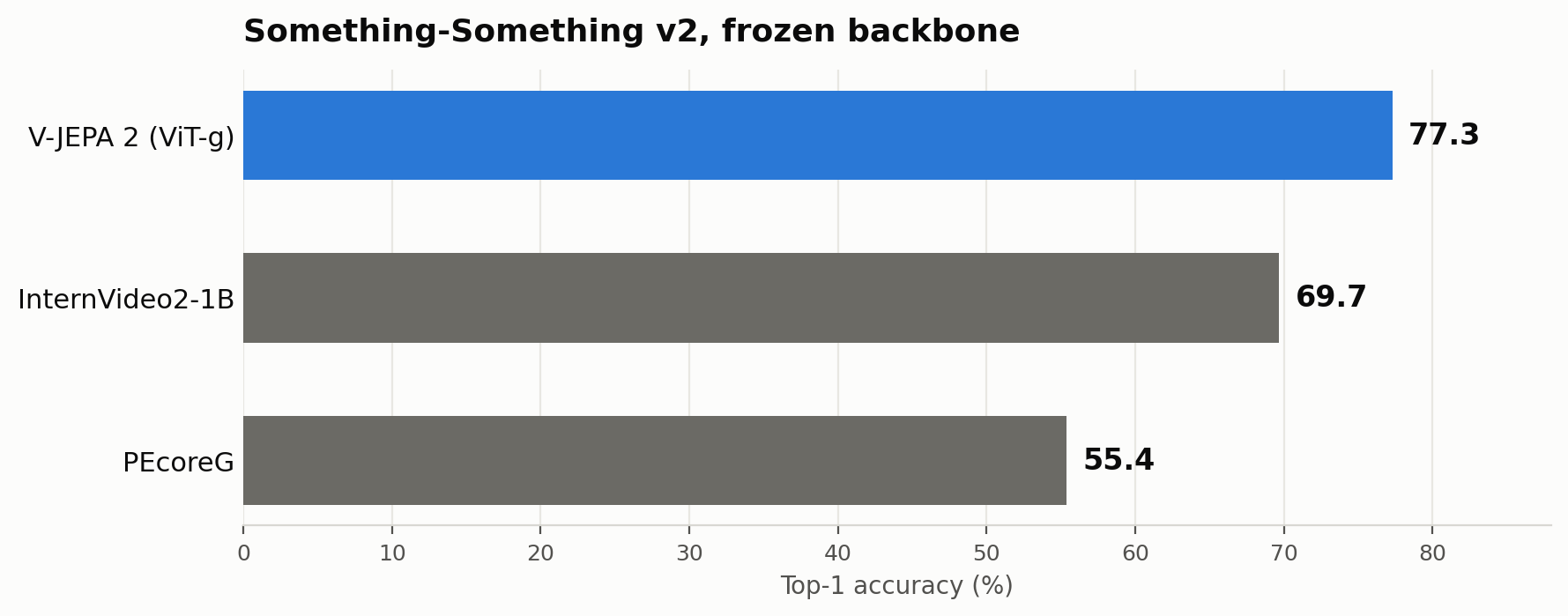 Figure 4: Something-Something v2 with a frozen backbone. The classes are things like “pushing something so it falls off the table”, so recognizing objects gets you nowhere; you have to have understood the motion. Source: Author
Sit with the anticipation number for a second. The task is to name the verb and the noun of an action one second before it happens, from head-mounted video. Nobody trained the model to do this. It was trained to describe hidden patches, and short-horizon prediction of the future fell out for free.
Is it actually a world model?
Here I want to be pedantic, because the marketing has run ahead of the architecture.
A world model needs a transition function, $s_{t+1} = f(s_t, a_t)$. Given where you are and what you do, where do you end up. Go back and look at what the JEPA predictor is conditioned on, and you will find position and nothing else. It answers “what’s over there”, not “what happens if I try this”.
Our witness can describe the room in beautiful detail. Ask her what’s through the door and she has nothing, because she never opened it.
| Tier | Predictor conditioned on | Examples | World model? |
|---|---|---|---|
| 1 | Nothing, no predictor at all | Pure joint-embedding methods | No, it’s a state space |
| 2 | Position, “what’s in this hole?” | I-JEPA, V-JEPA, V-JEPA 2 base | No, it’s latent inpainting |
| 3 | State and action, “what if I do X?” | V-JEPA 2-AC, DINO-WM, Dreamer | Yes |
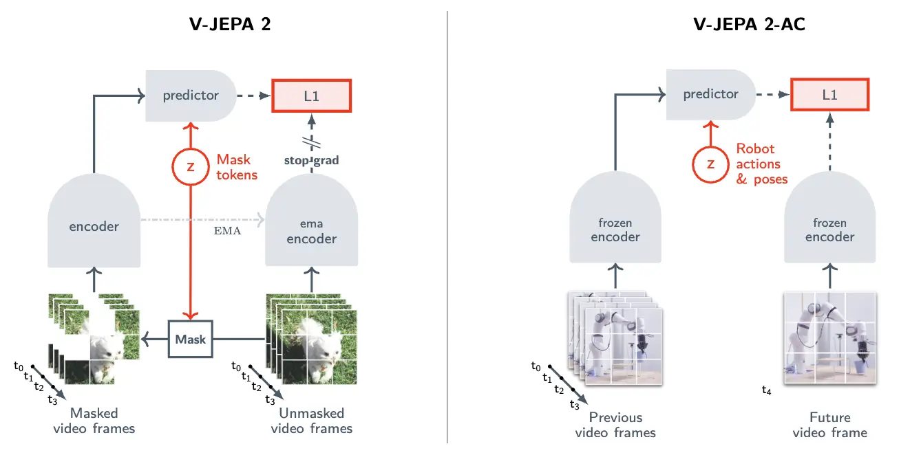 Figure 5: The whole argument in one picture. Same architecture, same $z$ slot. On the left $z$ carries mask tokens and you get latent inpainting; on the right $z$ carries robot actions and poses, the encoders are frozen, and you get a transition function. Source: V-JEPA 2
Which brings us to the part of the paper that earns the label. V-JEPA 2-AC freezes the encoder and post-trains a small action-conditioned predictor with block-causal attention on under 62 hours of unlabeled Droid robot video (a long weekend, if the robot skips sleep). Now there’s a real transition operator, so you can plan with it.
Planning is model-predictive control. Define the energy of a candidate action sequence as the L1 distance between the predicted future latent and the latent of a goal image:
\[a^*_{t:t+T} = \arg\min_{a_{t:t+T}} \; \big\| \hat{s}_{t+T}(a_{t:t+T}) - s_{\text{goal}} \big\|_1\]Optimize with the cross-entropy method, execute the first action, and replan, all of it in latent space, so no frame is ever drawn.
Deployed zero-shot on Franka arms in two labs with no data from either: roughly 80% pick-and-place, 75% reach-with-object, 65% grasp on cups and boxes. Octo manages 15% on grasp. Planning takes 16 seconds per action against about 4 minutes for Cosmos, which has to generate pixels in order to think (imagine having to paint a watercolour of the kitchen before you can decide to open the fridge).
And the line that settles it is in the ablation: action-unconditioned variants fail to infer control. With the same encoder, the same data and everything else unchanged, taking away the action conditioning means the world model stops being one, so tier 2 is not a smaller tier 3.
Why this matters
The useful lesson here is that the objective was the bottleneck, not the architecture. With the same transformers, the same data and the same compute, changing what you ask the model to predict makes the representations better and cheaper at once.
The payoff shows up in the frozen encoder. V-JEPA 2’s encoder doesn’t move during robot training at all, which is why 62 hours of interaction data is enough to get a working policy. The encoder already knows what a cup is, what “behind” means, and what falling looks like, because it watched a million hours of people doing things. Language models got their prior by reading the internet and we are running low on internet. Video is nowhere near exhausted.
The honest cons
Collapse is still managed by superstition. Everything above leans on an EMA teacher, a stop-gradient and a predictor kept weak on purpose, and not one of those is a proof. The degenerate solution is still sitting there at the bottom of the loss. We have just built enough scar tissue around it that gradient descent doesn’t wander in. Remove any single piece and training falls over, and nobody can tell you precisely why the remaining pieces are enough.
The evaluation protocol is doing real work too. Frozen probes are the right idea, but the attentive probe in these papers has four transformer blocks in it, so there’s a fair question about how much of 77.3 belongs to the encoder and how much to the probe. That one is not settled.
“World model” has become branding. Meta’s launch post calls V-JEPA 2 the first world model trained on video, which quietly folds the AC variant’s capability back onto a base model with no action conditioning anywhere in it. The base model is a representation learner. The 62 hours of post-training are what buy the name.
And when a JEPA is wrong, you can’t see it. A diffusion model that predicts the future hands you a picture you can look at and argue with. A JEPA hands you a 1024-dimensional vector that is wrong in some direction. V-JEPA ships a separate diffusion decoder purely so humans can inspect what the model believes, which is a debugging tool that got written up as a feature.
Conclusion
Stop painting the room. Describe it, predict the description, throw the wallpaper away. That’s the whole idea, and the benchmarks, the frozen encoders and a Franka arm in a lab that never saw its training data all say it works.
But look again at what’s holding it up: an EMA copy, a stop-gradient and a predictor hobbled on purpose, and every one of those exists to answer a question nobody could answer directly: what stops the witnesses from agreeing on nothing?
For five years the field could only say what a bad description looks like, and nobody could write down what a good one should look like. In late 2025 somebody did, and they brought a proof.
Stay tuned for part 2, where we meet LeJEPA, tear out the entire interrogation room, and replace it with a single term. Till then, ciao.