
On the cover: a poured melt, cored along two dozen random directions at once. Decorative, and also roughly what SIGReg does a thousand times a step.
Part 1 left us in an interrogation room. We had stopped asking models to repaint the scene and started asking them to describe it, we threw the wallpaper away, and the frozen-probe numbers said the trade was a good one.
Then we looked at what was holding the whole thing upright, and it was not pretty: an exponential moving average teacher, a stop-gradient, a predictor kept deliberately too weak to do the job alone, and a centering-and-sharpening schedule that somebody tuned during a conference deadline and nobody has touched since.
Not one of those forbids the model from answering “a person, probably” to every question ever asked of it. They make it unlikely, and the papers explaining why it is unlikely came out years afterwards, written by people who had been shipping it the whole time.
So the state of the art is a smithy. The master turns out genuinely beautiful blades, quenches at a temperature his grandfather picked, counts three hundred hammer blows because three hundred is the number, and could not tell you which part of that is load-bearing. Ask him and he will start talking about the moon. Somebody once tried two hundred and ninety and the billet cracked in the fire, so now nobody tries anything.
Welcome to the era of LeJEPA. This is the story of how somebody finally wrote down the spec sheet.
The charms are not free
It is tempting to file all this under aesthetics. The blades come out fine, the papers get published, so who cares if the recipe is folklore?
Accounting cares.
The charms are coupled: teacher decay interacts with the sharpening temperature interacts with the warmup length interacts with how narrow you made the predictor, so moving one means re-tuning the others. That is not a hyperparameter, it is a hyperparameter surface, and you cross-validate over it with runs that cost GPU-months. They also refuse to transfer. A recipe tuned for ViT-L on ImageNet is not a recipe for a ResNet on satellite imagery, and the failure mode is not “slightly worse”, it is a loss curve that goes flat on day two and stays flat.
Worse, you cannot read the training loss. In a teacher-student setup the loss falls whether the model is learning something or quietly collapsing toward the constant answer, so the only way to know if a run worked is to finish it, freeze the encoder, attach a probe and evaluate on labels. Self-supervised learning, whose entire pitch is that you do not need labels, could not tell you whether it was working without labels. It is a fuel gauge wired to the radio.
Which means the entry ticket was never the GPUs. It was the GPUs plus enough spare budget to set fire to a month, twice, before anyone could tell you if the recipe had taken.
The anatomy of a LeJEPA
Strip any joint-embedding method down and it is doing two jobs at once: pull the views of the same image together, and stop everything from piling into the same corner.
Family one from part 1 does the second job with machinery: the EMA copy, the stop-gradient, the crippled predictor. Barlow Twins and VICReg do it with statistics instead, and I said at the time to hold that thought.
Here it is. LeJEPA (Balestriero and LeCun, 2025) keeps the second family’s shape and replaces the hand-picked statistics with the one distribution you can prove is the right target:
\[\mathcal{L}_{\text{LeJEPA}} = (1-\lambda)\, \mathcal{L}_{\text{pred}} + \lambda\, \mathcal{L}_{\text{SIGReg}}\]where $\lambda \in (0,1)$ is the only knob in the objective. The prediction term is as plain as it gets: we take $V$ augmented views of an image, shove each one through the same encoder and projector to get $z_1 \dots z_V$, and pull each one toward the average of the others:
\[\mathcal{L}_{\text{pred}} = \frac{1}{V}\sum_{v=1}^{V} \big\| z_v - \bar{z} \big\|^2, \qquad \bar{z} = \frac{1}{V}\sum_{u=1}^{V} z_u\]Look at $\bar{z}$ for a second. It is not detached. Gradients flow back through every view, including the one being used as the target, which is precisely the thing every method since BYOL said you must never do.
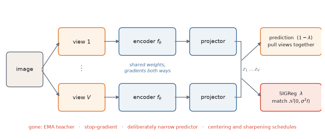 Figure 1: LeJEPA. One encoder, used on every view, with gradients flowing through all of them. Everything listed along the bottom used to be mandatory. The second loss term is what replaced the lot. Source: Author
NOTE: the second term operates on the projector output, not the encoder output. The features you actually keep and use downstream sit one layer upstream of the thing being made Gaussian. Everybody in this family does that, and nobody has a clean story for why it helps.
What a good description should look like
You are casting a part and the drawing does not say what it gets bolted to. Might be a hinge, might be a bracket taking a load straight down, might be something the customer has not designed yet and will phone you about on a Friday. All you know is how much metal is in the crucible.
What shape do you pour?
Whatever else you pour, you do not pour a long thin one. Pour a wire and the first load that turns up off-axis snaps it, and nobody in the subsequent meeting will accept “the load came from the wrong direction” as an answer. You pour the thing that is equally strong whichever way it gets pulled, because you are not in a position to bet on a direction. That, in overalls, is what the paper proves.
Formally, fix the trace of the embedding covariance, since otherwise you can cheat by making everything bigger. Over the downstream tasks you might face, the isotropic Gaussian $\mathcal{N}(0, \sigma^2 I)$ then uniquely minimises the integrated bias of linear, kernel and $k$-NN probes. Isotropy handles the direction gamble; Gaussianity handles the variance term, and it is the maximum-entropy distribution for a given covariance, which is to say it commits to nothing you did not ask for.
Brace yourselves, here is the arithmetic that makes it concrete.
Take a 512-dimensional embedding and a variance budget of 512 units. Cast A puts 64 units into each of 8 directions and zero into the remaining 504. Cast B puts 1 unit into every direction. Now a downstream task shows up needing to read off some direction $w$ that you did not know about at training time. Under Cast A, the chance that $w$ lands anywhere near the 8 directions carrying signal is about 1.6%, and in the other 98.4% of cases your probe is reading a constant and learning nothing. Under Cast B, every direction it could possibly ask for has variance 1.
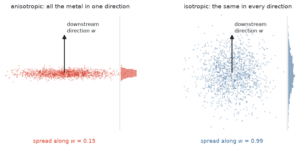 Figure 2: The same amount of metal, poured two ways. Both clouds have the same total variance. The flat one has 0.15 of spread along the direction the downstream task happened to want; the round one has 0.99, and would have 0.99 along any other direction you picked. Source: Author
Real anisotropy is graded rather than binary, so in practice the numbers are less lurid than 1.6%, though the ordering survives every version of the calculation I tried.
SIGReg, or: you cannot X-ray an ingot
Fine, so we aim for the isotropic Gaussian. Now how do we check whether we got there, you ask?
This is where it should fall apart. Testing whether a cloud of points in 512 dimensions follows a particular multivariate distribution is a famously hopeless problem, the batch you are testing has maybe 512 points in it, and you need to do this on every step of training for a hundred epochs.
The way out was published in 1936 by two statisticians with, I am confident, no GPUs between them. Cramér–Wold says a distribution on $\mathbb{R}^D$ is completely determined by the distributions of its one-dimensional projections $w^\top z$ over all unit vectors $w$. Which specialises to exactly what we need: $z$ is isotropic Gaussian if and only if every one of its 1D shadows is the same univariate $\mathcal{N}(0, \sigma^2)$, whichever way you point.
You cannot X-ray the ingot, but you can take core samples, and if every core comes out right, so does the ingot.
Step 1: the core sample
We draw $K$ random directions, sample them Gaussian and normalise each to unit length, and stack them into $A \in \mathbb{R}^{D \times K}$. Then we project the batch, $P = ZA$, which is one matmul. $K$ is 1024 in the paper’s ImageNet configs and 256 in their minimal example.
We obviously cannot check every direction, there are infinitely many, so we draw a fresh $K$ of them on every step, seeded off the global step so that all GPUs pick the same ones. Over a run you cover the sphere in expectation, and the model never gets to learn which directions the inspector prefers (models, like students, study for the exam they expect).
Step 2: tap it and listen
Now the univariate test. The characteristic function of a distribution is its Fourier transform, $\varphi(t) = \mathbb{E}[e^{itX}]$, and you can think of it as the sound a sample makes when you tap it: two distributions are identical exactly when they ring the same at every frequency. For the standard normal the ring is $\varphi(t) = e^{-t^2/2}$, which is clean and known in advance and needs no estimating.
The Epps–Pulley statistic measures the gap between the sample’s ring and that one. In words first:
\[T = N \times \sum_{\text{frequencies}} \big(\text{how far off the sample rings there}\big)^2 \times \big(\text{how much that frequency counts}\big)\]specifically,
\[T = N \int \big| \hat{\varphi}(t) - e^{-t^2/2} \big|^2 \, e^{-t^2/2} \, dt\]where $N$ is the number of samples, $\hat{\varphi}(t) = \frac{1}{N}\sum_{n=1}^{N} e^{i t p_n}$ is the empirical characteristic function of the projected values $p_n$, and the second $e^{-t^2/2}$ is the weight, which says low frequencies count for more than high ones.
In the implementation that integral is a sum over 17 points between $t=0$ and $t=3$, exploiting the symmetry of the real and imaginary parts to do half the arithmetic. Seventeen. Not sixteen, not twenty. Somebody ran the ablation over 5, 17 and 41 and came back with 17, and I have more faith in that number than in any round one.
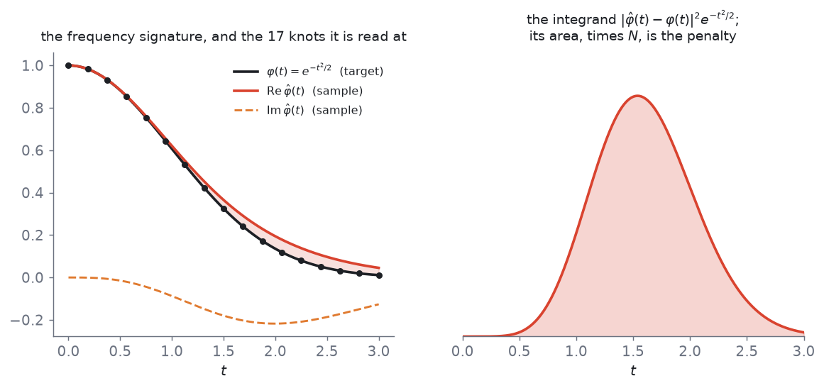 Figure 3: Left, the standard normal’s frequency signature in black and a projected sample’s in red, read at 17 points. Right, the weighted squared gap between them. Its area, times the batch size, is what gets added to the loss. Source: Author
The library ships Anderson–Darling, Cramér–von Mises, Shapiro–Wilk, Jarque–Bera and Watson too, so picking Epps–Pulley was a decision. It is built from $\cos$ and $\sin$ of the data, and those are bounded, so the loss and its gradient are bounded. Kolmogorov–Smirnov makes no such promise, and an unbounded penalty on a live minibatch is a spike waiting to happen. Running a normality test once on a finished dataset and differentiating through one four hundred thousand times are not the same job.
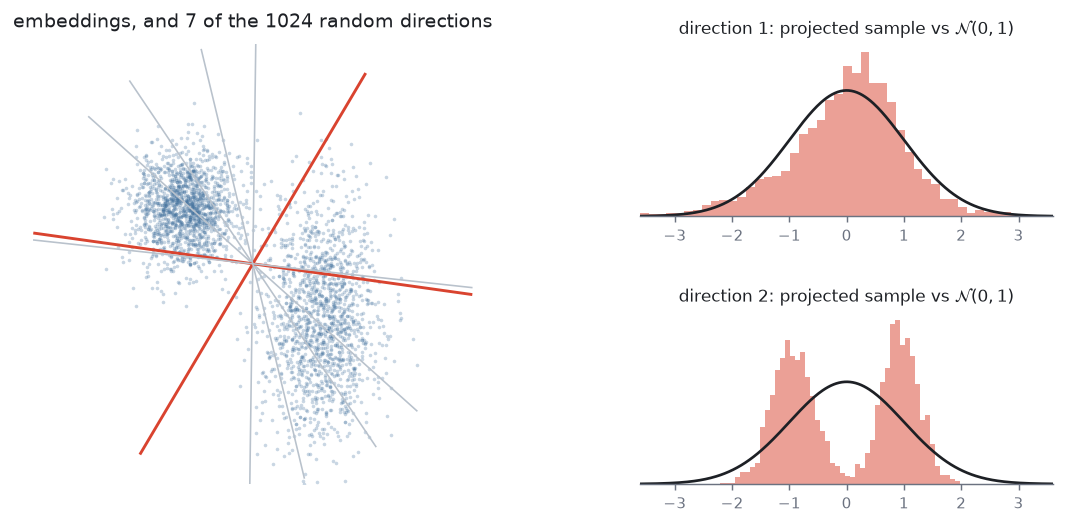 Figure 4: Slicing in action. Direction 1 gives a projection that passes for Gaussian and contributes almost nothing to the loss. Direction 2 catches the same cloud being two lumps and is where the gradient comes from. Source: Author
Step 3: the dial
Average the statistic over the $K$ directions, multiply by $\lambda$, add the prediction term times $(1 - \lambda)$, and you have the objective. $\lambda$ is 0.05 in the ImageNet runs and 0.02 in the small one. Fifty lines, one number to pick, and I have watched grown engineers lose a fortnight to six.
There is a detail here I keep coming back to. To compute the statistic across a global batch spread over hundreds of GPUs, the only things that have to cross the wire are the per-knot means of $\cos(t p_n)$ and $\sin(t p_n)$. That is 34 floats per direction, whether the global batch is 512 images or 512,000. The test comes out exact over every sample on every device for less traffic than your laptop spends telling a server it is still awake.
What that buys
The paper reports the recipe running out of the box across 60+ architectures, ResNets and ViTs and ConvNets, 10+ datasets, and up to 1.8B parameters, with no per-architecture tuning and no gradient clipping.
Here is the head-to-head against part 1’s I-JEPA, averaged over eight transfer datasets at three labelling budgets:
| Model | Params | Epochs | 1-shot | 10-shot | all labels |
|---|---|---|---|---|---|
| LeJEPA ViT-L | 304M | 100 | 29.55 | 60.95 | 79.48 |
| LeJEPA ConvNeXtV2-H | 660M | 100 | 31.58 | 60.70 | 77.56 |
| I-JEPA ViT-H | 632M | 300 | 30.20 | 60.51 | 78.50 |
Nobody wins that table. The margins are under a point and I would not defend a single one of them, and that is exactly the point: half the parameters, a third of the epochs, the whole apparatus of part 1 gone (teacher, stop-gradient, predictor and schedules), and the result is a tie. Scale it up and a ViT-H/14 gets 79% on ImageNet-1K under a frozen linear probe, against DINOv2’s ViT-g/14 at 86.5%. Seven and a half points is not a rounding error and nobody pretends it is.
The number I would actually build on is a different one. The training loss correlates with downstream probe accuracy at 94%+ Spearman. You can pick a model by looking at the loss, before the run has finished and without a single label, instead of waiting three days to find out it was dead on Tuesday. After five years of a number on a screen that told you nothing, somebody wired the gauge to the tank.
Which drops the price of admission. Their worked example gets a ViT-S/8 to 90.7% on Imagenette in about 200 minutes on one GPU. And in-domain pretraining stops being a doomed move: on Galaxy10, roughly 11k pictures of galaxies, training from scratch beats transferring from DINOv2. Eleven thousand images beat a model that ate the internet, and I read that table twice to be sure.
| Piece | I-JEPA and friends | LeJEPA | What it was for |
|---|---|---|---|
| Target encoder | EMA copy, $\tau \approx 0.996$–$0.999$ | none | stopping the branches agreeing on nothing |
| Gradient path | stop-grad on the target | gradients through all views | same |
| Predictor | narrow ViT, weak on purpose | none | same |
| Output schedule | centering and sharpening | none | same |
| What forbids collapse | nothing, empirically | the SIGReg term | — |
| Knobs in the loss | several, coupled | one, $\lambda$ | — |
And the ablation is one you can run in your head. Set $\lambda = 0$ and the prediction term is on its own, and its global minimum is the constant embedding, which is part 1’s representation collapse turning up right on cue. These models are lazy animals. Leave a free lunch in the loss and gradient descent will have found it before you have finished typing wandb.init. What is different is that you can see it coming from the algebra rather than from a dead run on Thursday morning.
Where things are going
LeWorldModel (2026): LeWorldModel drops SIGReg into an action-conditioned world model trained end to end from pixels, with a next-embedding prediction loss and the Gaussian regulariser as its only two terms. Six tunable loss hyperparameters down to one against the previous end-to-end alternative, about 15M parameters on a single GPU, planning up to 48x faster than world models built on foundation backbones. That is part 1’s tier 3 reached without the machinery, and the cheap end of the world-models-as-data-substrate bet the VLA post closed on. When Does LeJEPA Learn a World Model? then asks the question part 1 spent a whole section being pedantic about, and asks it as a conditional rather than a slogan.
Arguing with the target: the isotropic Gaussian is now something people push back on, which is good, since you can only argue with a target once somebody has named one. Beyond Isotropy in JEPAs proposes a Hamiltonian geometry instead, SPHERE-JEPA goes to the sphere, KerJEPA swaps the characteristic-function test for kernel discrepancies. People arguing about whether the target is right is a much better problem to have than the previous one, where there was no target to argue about and everyone just added another trick.
Video: LeVJEPA carries the recipe to clips, where the compute savings compound, since video is where the heuristic-tuning bill was always worst.
What is still folklore
SIGReg constrains the shape of the cloud, and says nothing whatsoever about what should count as two views of the same image. That question is still answered the way it was in 2021: 2 global crops, 6 local crops, colour jitter, grayscale, blur, solarisation, every threshold and probability inherited from DINO and none of them re-derived. Each of those numbers is somebody’s Tuesday afternoon. Given a choice of which half to put on a proof, I would have picked that one.
Seven and a half points behind DINOv2 also settles who this is for. If you want the best frozen ImageNet features on earth, go and download DINOv2, it is right there and it is free. LeJEPA is for when nobody has pretrained on your data and nobody is going to, because your data is 11,000 galaxies or a radiology archive you cannot upload anywhere.
The sliced test is weaker in high dimensions than the Cramér–Wold theorem makes it sound. Random 1D projections of almost any high-dimensional distribution drift toward Gaussian as $D$ grows, a result Diaconis and Freedman made precise in 1984, which means a cloud can sail through a great many 1D normality tests while being badly non-Gaussian in ways no single direction reveals.
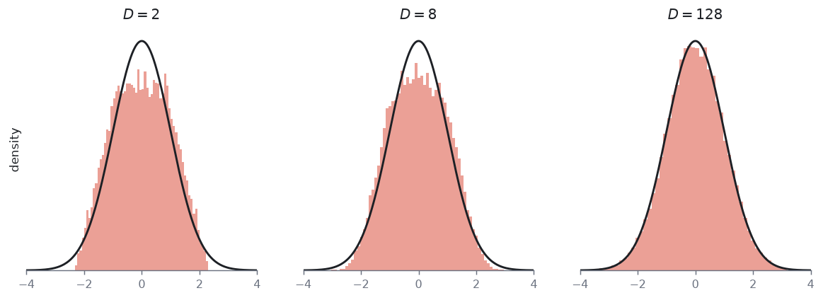 Figure 5: Points drawn uniformly from a hypercube, which is about as un-Gaussian as a distribution gets, projected onto one random direction. At $D=2$ the test would catch it instantly. At $D=128$ the projection is visually indistinguishable from the bell curve it is being compared against. Source: Author
The theorem still holds, since it quantifies over all directions and you are sampling 1024 of them fresh each step. The paper’s answer is that embeddings from a smooth network are not adversarial, so a modest number of slices has real power. I believe that and I would still like to see somebody map the failure mode instead of arguing about it.
And “provable” describes the target, not the trip. The theorem says an isotropic Gaussian embedding minimises downstream risk. It does not say gradient descent on this penalty arrives at one, and there is no convergence guarantee here. All that changed is that the objective now names the place it is trying to reach, which beats an objective whose easiest answer is the disaster.
Conclusion
Part 1 argued that reconstruction was the wrong thing to ask for: describe the room, do not repaint it, nobody cares about the wallpaper. It also admitted it could not say what a good description was, only that you knew a bad one when you were looking at it.
This is the other half of that. A good description spreads itself out evenly, because the job you will eventually be asked to do points somewhere nobody has told you about yet, and anything you piled up in one direction was a bet you did not have to make. You can prove it, and acting on it costs one extra term and about fifty lines of Python. The teacher network, the stop-gradient and the predictor kept weak on purpose turn out to have been packing material stuffed around the gap where that sentence should have been.
The smith still makes the blade, and it is still a good blade. He has just stopped doing it at midnight, and the next time an apprentice asks him why three hundred, somebody in the room can answer.
And now you know. Fin.